1 Capacitor
(written test, approx. 12 % of a 120-minute written test, SS2024)
Older capacitive pressure sensors are based on a parallel plate capacitor setup (see left-side image).
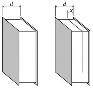
In the following such a sensor is given with:
- Plate area : $A=25 ~\rm mm^2$
- Distance between both plates: $d=200 ~\rm \mu m$
- Air between the plates: $\varepsilon_{\rm r,air}=1$
- Supply voltage: $3.3 ~\rm V$
- Boundary effects on the end of the layers shall be ignored in the following calculations.
$\varepsilon_{0} =8.854 \cdot 10^{-12} ~\rm F/m $
1. Calculate the capacity $C$.
2. Calculate the value of the displacement field between the plates, when a voltage of $U=3.3 ~\rm V$ is applied.
3. Calculate the charge difference between both plates for a voltage of $U=3.3 ~\rm V$.
4. Due to a production problem, the right-side layer is covered with a contaminant, see the right-side image.
The contaminant has $\varepsilon_{\rm r,c}>\varepsilon_{\rm r,air}$, while the distance between the plates remains the same.
Give a generalized formula $C_2=f(A,d,x,\varepsilon_{\rm r,c}, \varepsilon_{\rm r,air})$.
Therefore: \begin{align*} C = {{1}\over{ {{1}\over{C_{\rm air} }} + {{1}\over{ C_{\rm c}}} }} \end{align*}
With \begin{align*} C_{\rm air} &= \varepsilon_0 \varepsilon_{\rm r, air} {{A}\over{d-x}} &&= \varepsilon_0 A {{\varepsilon_{\rm r, air}}\over{d-x}} \\ C_{\rm c} &= \varepsilon_0 \varepsilon_{\rm r, c} {{A}\over{x}} &&= \varepsilon_0 A {{\varepsilon_{\rm r, c} }\over{x}} \\ \end{align*}
This leads to: \begin{align*} C = \varepsilon_0 A {{1}\over{ {{d-x}\over{\varepsilon_{\rm r, air} }} + {{x}\over{ \varepsilon_{\rm r, c}}} }} \end{align*}