4 Analysis of Networks

Network analysis plays a central role in electrical engineering. It is so important because it can be used to simplify what at first sight appear to be complicated circuits and systems to such an extent that they can be understood and results derived from them.
In addition, networks also occur in other areas, for example, the momentum flux through a truss or the heat flux through individual hardware elements (Abbildung 1, or an example for heat flow through electronics). The concepts shown below can also be applied to these networks.
On the wiki page for network analysis the different methods are described very well in a compact way
Learning Objectives
By the end of this section, you will be able to:
determine the number of nodes, number of (tree and connecting) branches, and number of meshes.construct a complete tree from an electrical network.understand the mesh current method and node potential method.- understand and be able to apply the superposition procedure.
4.1 Preliminary Work for Network Analysis
Preparation of the Circuit

Before the network analysis can be tackled, the circuit must be suitably prepared (cf. Abbildung 2):
- Clarify what is given and what is sought
- Draw a circuit
- Add voltage and current arrows. If not already given, then:
- First, draw current and voltage arrows at all sources according to the generator arrow system.
- Afterwards, define the current arrows at the remaining branches as you like.
- Finally, draw the voltage arrows at the loads according to the load arrow system.
- Select suitable current and voltage designations. If not already given, then:
- Count indices continuously, i.e. one number per element (source or load).
- Do not insert any signs in front of the designators in the circuit.
In real applications, it is useful to specify the number of variables („what is wanted?“), parameters („what can be adjusted?“, e.g. potentiometer) and known quantities („what is given?“).
This makes it clear how many equations are needed. This seems to become difficult for larger networks - but a trick for this is presented below.
It often helps to draw the drawing several times (at least in your head) to have enough space for the identifiers (cf. Abbildung 2 below).
Graphs and Trees

In the chapter 2. simple dc_circuits the terms nodes, branches, and loops have already been explained. These will now be expanded here to better explain the various network analysis methods in the following. In Abbildung 3 the graph of the example network is drawn. We had already seen this one too, but without knowing that this is called a graph!
But the important thing is: In this graph, only the (real) nodes are drawn. Nodes are by definition the connection of more than two branches. Accordingly, the connection between $R_{10}$ and $R_7$ is not a node 1) ! For this reason, also the blue circle as a sign for nodes is omitted here.
A concept that has not yet appeared is that of the complete tree. For this, some (mathematical) graph theory is needed. There, too, the terms nodes and loops are used as before. A tree here is a special kind of graph. The graph in Abbildung 3 shows several loops.
Now a tree is characterized precisely by the fact that it contains no loops. Three different trees are drawn in the picture. From a given network, many different trees can be created (depending on the number of nodes).
Among the different trees, there are now some in which each node connects two or fewer loops. 2) These are called complete trees (occasionally also Hamiltonian path ). Complete trees can also be understood as this shows a path through the network where all nodes are visited only exactly once.
Tree 3 in Abbildung 3 is now just one of the possible complete trees of this network.
The branches in complete trees are now distinguished according to their membership:
- tree branches belong to the complete tree (solid lines in Abbildung 3).
- Connecting branches do not belong to the complete tree (dotted lines in Abbildung 3).
Why does the excursion to graph theory make sense now? The trick is that by defining the complete tree, all loops have just been removed. Conversely, a new (independent) loop can be created by each connecting branch. So if the number of independent loop equations $m$ is sought, this is just equal to the number of connecting branches.
To do this, proceed as follows:
- Determine the number of (real) nodes $k$.
- Determine the number of branches $z$
- The number of tree branches $b$ is now $k-1$. (each node is traversed only once; at the last node there is no further branch).
- The number of connecting branches $v$ is given by „All branches minus tree branches“: $v = z - b = z - k + 1$
Thus, the number of independent loop equations $m$ is findable by counting the nodes $k$ and branches $z$ over $m = v = z - k + 1$.
This explanation can also be heard again in this video and is explained again clearly via this video.
4.2 Branch Current Method

The branch current method (also called branch current method) now „simply times“ (almost) all equations of the circuit. Specifically, for each node and each independent loop, the node and loop equations are written down:
- for all nodes $k$ respectively the equation: $\sum_{k=0}^{N_k}{I_k}=0$
- for all independent loops $m$ respectively the equation: $\sum_{m=0}^{N_m}{U_m}=0$
Here the number $m$ (as mentioned in the previous subsection) can be determined by the number of nodes and branches.
This forms a linear system of equations. This can then be considered as a matrix equation and solved with the rules of (mathematical) art.
For the example (Abbildung 4), these would be the equations:
The matrices still need to be corrected for the voltage and current sources!!!
Example of nodal equations
\begin{align*} \sum\limits_{k=0}^{N_k}{I_k}=0 \end{align*}
Setting up the individual equations: \begin{align*} \scriptsize\text{node 'a'} & \scriptsize : -I_0 - I_9 - I_7 = 0 \\ \scriptsize\text{node 'b'} & \scriptsize : +I_0 - I_1 - I_3 = 0 \\ \scriptsize\text{node 'c'} & \scriptsize : + I_1 - I_2 - I_4 = 0 \\ \scriptsize\text{node 'd'} & \scriptsize : - I_5 + I_4 - I_{11} = 0 \\ \scriptsize\text{node 'e'} & \scriptsize : + I_5 + I_6 - I_7 = 0 \\ \scriptsize\text{node 'f'} & \scriptsize : - I_2 + I_3 - I_6 + I_9 + I_{11} = 0 \\ \end{align*}
Sorting currents into columns: \begin{align*} \begin{smallmatrix} \text{node 'a'}: & -I_0 & & & & & & & - I_7 & - I_9 & & = 0 \\ \text{node 'b'}: & +I_0 & - I_1 & & - I_3 & & & & & & = 0 \\ \text{node 'c'}: & & + I_1 &- I_2 & & - I_4 & & & & & = 0 \\ \text{node 'd'}: & & & & + I_4 & - I_5 & & & - I_{11} & = 0 \\ \text{node 'e'}: & & & & & + I_5 & + I_6 & - I_7 & & = 0 \\ \text{node 'f'}: & & & - I_2 & + I_3 & & - I_6 & & + I_9 & + I_{11} & = 0 \\ \end{smallmatrix} \end{align*}
Setting up the matrix: \begin{align*} \left( \begin{smallmatrix} -1 & 0 & 0 & 0 & 0 & 0 & 0 & -1 & -1 & 0 \\ +1 & -1 & 0 & -1 & 0 & 0 & 0 & 0 & 0 & 0 \\ 0 & +1 & -1 & 0 & -1 & 0 & 0 & 0 & 0 & 0 \\ 0 & 0 & 0 & 0 & +1 & -1 & 0 & 0 & 0 & -1 \\ 0 & 0 & 0 & 0 & 0 & +1 & +1& -1 & 0 & 0 \\ 0 & 0 & -1 & +1 & 0 & 0 & -1& 0 & +1 & +1 \\ \end{smallmatrix} \right) \cdot \left( \begin{smallmatrix} I_0 \\ I_1 \\ I_2 \\ I_3 \\ I_4 \\ I_5 \\ I_6 \\ I_7 \\ I_9 \\ I_{11} \end{smallmatrix} \right) = \vec{0} \end{align*}
Example of loop equations
\begin{align*} \sum\limits_{m=0}^{N_m}{U_m}=0 \end{align*}
Setting up the individual equations: \begin{align*} \scriptsize\text{Masche 'abf'} & \scriptsize : -U_0 + U_3 - U_9 = 0 \\ \scriptsize\text{Masche 'bcf'} & \scriptsize : +U_1 - U_2 - U_3 = 0 \\ \scriptsize\text{Masche 'cdf'} & \scriptsize : + U_2 + U_4 - U_{11} = 0 \\ \scriptsize\text{Masche 'def'} & \scriptsize : + U_5 - U_6 + U_{11} = 0 \\ \scriptsize\text{Masche 'eaf'} & \scriptsize : + U_6 - U_7 - U_{10} + U_9 = 0 \\ \quad \\ \end{align*}
Sorting voltages into columns: \begin{align*} \begin{smallmatrix} \text{Masche 'abf'}: &-U_0 & & & + U_3 & & & & & & - U_9 & & & = 0 \\ \text{Masche 'bcf'}: & & + U_1 & - U_2 & - U_3 & & & & & & & & & = 0 \\ \text{Masche 'cdf'}: & & & + U_2 & & + U_4 & & & & & & & - U_{11}& = 0 \\ \text{Masche 'def'}: & & & & & & + U_5 & - U_6 & & & & & + U_{11} & = 0 \\ \text{Masche 'eaf'}: & & & & & & & + U_6 & - U_7 - U_{10} & & - U_9 & & & = 0 \\ \quad \\ \quad \\ \end{smallmatrix} \end{align*}
Set up the matrix, but note $U_m = R_x \cdot I_m$: \begin{align*} \left( \begin{smallmatrix} -R_0 & 0 & 0 & +R_3 & 0 & 0 & 0 & -R_9 & 0 & 0 \\ 0 & +R_1 & -R_2 & -R_3 & 0 & 0 & 0 & 0 & 0 & 0 \\ 0 & 0 & +R_2 & 0 & +R_4 & 0 & 0 & 0 & 0 & -R_{11} \\ 0 & 0 & 0 & 0 & 0 & +R_5 &-R_6 & 0 & 0 & +R_{11} \\ 0 & 0 & 0 & 0 & 0 & 0 &+R_6 &-R_7-U_{10}& -R_9 & 0 \\ \end{smallmatrix} \right) \cdot \left( \begin{smallmatrix} I_0 \\ I_1 \\ I_2 \\ I_3 \\ I_4 \\ I_5 \\ I_6 \\ I_7 \\ I_9 \\ I_{11} \end{smallmatrix} \right) = \vec{0} \quad \\ \end{align*}
These matrices can be solved using, for example, the Gaussian elimination.
Another example in videos
In video 1 you will learn:
1. writing down the given circuit and sizes
2. drawing in and designating the nodes
3. draw in and label the loops
4. draw and label the mesh currents
5. drawing in and designating the mesh voltages
for a simple circuit
Mesh current analysis Example 1/3
In video 2 you will learn :
1. writing down the given circuit and sizes
2. drawing in and designating the nodes
3. draw in and label the loops
4. draw and label the branch currents
5. drawing in and designating the branch voltages
for a more complex circuit
Branch current analysis 2/3
Video 3 describes the following steps:
1. write down the given circuit and sizes
2. draw in and designate the nodes
3. draw in and label the loops
4. draw and label the branch currents
5. draw in and designate the branch voltages
6. set up node equations and loop equations
7. convert to matrix notation
8. solve the matrix
Mesh current analysis 3/3
In the Video 4 (not embedded here), will teach you how to solve a matrix by using a calculator:
9. inserting the numerical values into a calculator
10. calculating the matrix with a calculator
Exercise 4.2.1
4.3 Mesh Current Method
In the mesh current method, only for all loops $m$ each equation: $\sum\limits_{j=0}^{N_j}{U_j}=0$ are considered. However, these are represented in the form $R\cdot I = U $.
The advantage here is that the number of equations to be solved is reduced to the number of independent loop currents.
These can also be considered matrix equations and can be solved with the rules of (mathematical) art.
In video 1, the mesh current method is applied using an example.
mesh current method
Also in video 2, the mesh current method is applied using an example.
mesh current method
In the Video 3 (not embedded here) shows in detail how the loop current method can be derived.
4.4 Nodal Potential Method
In the nodal potential method, only the equation: $\sum\limits_{i=0}^{N_i}{I_i}=0$ are considered for all nodes k respectively. However, these are expressed in the form ${1\over R} \cdot U = I $ and $G \cdot U = I $ respectively.
The advantage here is that the number of equations to be solved is reduced to the number of existing nodes (minus 1).
These can also be considered matrix equations and can be solved with the rules of (mathematical) art.
In Video 1, the idea behind node potential analysis is simply explained.
Simple example of node potential analysis
Video 2 also uses the nodal potential method with an example.
more complex example of a node potential analysis
In the Video 3 (not embedded here) shows in detail how the nodal potential method can be derived.
4.5 Superposition Method / Superposition Principle
The superposition principle shall first be illustrated by some examples:
Example 1 - from an interview of a consulting company
Task: Three students are to fill a pool. If Alice has to fill it alone, she would need 2 days. Bob would need 3 days and Carol would need 4 days. How long would it take all three to fill a pool if they helped together?
The question sounds far off-topic at first but is directly related. The point is that to solve it, filling the pool is assumed to be linear. So Alice will fill $1 \over 2$, Bob $1 \over 3$, and Carol $1 \over 4$ of the pool per day. So on the first day, ${1 \over 2}+{1 \over 3}+{1 \over 4} = {{6 + 4 + 3} \over 12} = {13 \over 12}$ of the pool filled.
So the three of them need ${12 \over 13}$ of a day.
However, this solution path is only possible because in linear systems the partial results can be added.
Example 2 - Spring Force and Displacement

Task:A mechanical, linear spring is displaced due to masses $m_1$ and $m_2$ in the Earth's gravitational field (see Abbildung 5). What is the magnitude of the deflection if both masses are attached simultaneously?
Again, a linear law is used here: \begin{align*} \vec{s}= f(\vec{F}) = - D \cdot \vec{F} \end{align*}
The (seemingly trivial) approach applies here: \begin{align*} \vec{s}_{1+2} = f(\vec{F_1} + \vec{F_2}) &= - D \cdot (\vec{F_1} + \vec{F_2}) \\ &= - D \cdot \vec{F_1} - D \cdot \vec{F_2} \\ &= f(\vec{F_1}) + f(\vec{F_2}) \\ &= \vec{s_1} + \vec{s_2} \end{align*}
Notice:
In a physical system in which effect and cause are linearly related, the effect of each cause can first be determined separately. The total effect is then the sum of the individual effects.For electrical engineering this principle was described by Hermann_von_Helmholtz:
The currents in the branches of a linear network are equal to the sum of the partial currents in the branches concerned caused by the individual sources.
Thus, in the superposition method, the current (or voltage) sought in a circuit with multiple sources can be viewed as a superposition of the resulting currents (or voltages) of the individual sources.
The „recipe“ for the overlay is as follows:
- Choose the next source
x - Replace all ideal sources with their respective equivalent resistors:
- ideal voltage sources by short circuits
- ideal current sources by an open line
- Calculate the partial currents sought in the branches considered.
- Go to the next source
x=x+13), and to point 2, as long as the partial currents of all sources have not been calculated. - Add up the partial currents in the branches under consideration, observing the correct sign.
This procedure is explained again in more detail using examples in the two videos on the right.
Simple view of the superposition principle
A more complex example of the superposition method
Example
Abb. 6: example circuit with superposition 
Introduction to Nodal, Mesh and Superposition Method
Exercises
Exercise E4.5.1 Converting a bipolar signal to a unipolar signal (not from written test)
Imagine you want to develop a circuit that conditions a sensor signal so that it can be processed by a microcontroller. The sensor signal is in the range $U_{\rm sens} \in [-15...15~\rm V]$, and the microcontroller input can read values in the range $U_{\rm uC} \in [0...3.3~\rm V]$. The sensor can supply a maximum current of $I_{\rm sens, max}=1~\rm mA$. For the internal resistance of the microcontroller, input applies: $R_{\rm uC} \rightarrow \infty$
For conditioning, the input signal is to be fed via the series resistor $R_3$ to the center potential of a voltage divider $R_1 - R_2$ with $R_1$ to a supply voltage $U_{\rm s}$.
The following simulation shows roughly the situation (the resistor values are not correct).
Questions:
1. Find the relationship between $R_1$, $R_2$, and $R_3$ using superposition.
- Determine suitable values for $R_1$, $R_2$, and $R_3$.
- What values for $R^0_1$, $R^0_2$, and $R^0_3$ from the E24 series can be used to do this?
To make the calculation simpler, the resistors $R_3$ and $R_{\rm s}$ will be joined to $R_4 =R_3 +R_{\rm s}$.
Circuit 1 : only consider $U_{\rm S}$, ignore $U_{\rm I}$

\begin{align*} U_{\rm O}^{(1)} &= U_{\rm S} \cdot {{R_2||R_4}\over{R_1 + R_2||R_4}} = U_{\rm S} \cdot {{ {{R_2 R_4}\over{R_2 + R_4}} }\over{R_1 + {{R_2 R_4}\over{R_2 + R_4}} }} \\ &= U_{\rm S} \cdot {{ R_2 R_4 }\over{R_1 (R_2 + R_4)+ R_2 R_4 }} \\ &= U_{\rm S} \cdot {{ R_2 R_4 }\over{R_1 R_2 + R_1 R_4 + R_2 R_4 }} \\ \end{align*}
Circuit 2 : only consider $U_{\rm I}$, ignore $U_{\rm S}$

\begin{align*} U_{\rm O}^{(2)} &= U_{\rm I} \cdot {{R_1||R_2}\over{R_4 + R_1||R_2}} = U_{\rm I} \cdot {{ {{R_1 R_2}\over{R_1 + R_2}} }\over{R_4 + {{R_1 R_2}\over{R_1 + R_2}} }} \\ &= U_{\rm I} \cdot {{ R_1 R_2 }\over{R_4 (R_1 + R_2)+ R_1 R_2 }} \\ &= U_{\rm I} \cdot {{ R_1 R_2 }\over{R_4 R_1 + R_4 R_2+ R_1 R_2 }} \\ \end{align*}
Superposition: Let's sum it up!
These two intermediate voltages for the single sources have to be summed up as $U_{\rm O}= U_{\rm O}^{(1)} + U_{\rm O}^{(2)}$.
When deeper investigated, one can see that the denominator for both $U_{\rm O}^{(1)}$ and $U_{\rm O}^{(2)}$ is the same.
We can also simplify further when looking at often-used sub-terms (here: $R_2$)
\begin{align*} U_{\rm O} &= {{ 1 }\over{R_4 R_1 + R_4 R_2+ R_1 R_2 }} \cdot (U_{\rm S} \cdot R_2 R_4 + U_{\rm I} \cdot R_1 R_2 ) \\ U_{\rm O} \cdot (R_4 R_1 + R_4 R_2+ R_1 R_2 ) &= U_{\rm S} \cdot R_2 R_4 + U_{\rm I} \cdot R_1 R_2 \\ \\ U_{\rm O} \cdot ({{R_1 R_4}\over{R_2}} + R_4 + R_1 ) &= U_{\rm S} \cdot R_4 + U_{\rm I} \cdot R_1 \tag 1 \\ \end{align*}
The formula $(1)$ is the general formula to calculate the output voltage $U_{\rm O}$ for a changing input voltage $U_{\rm I}$, where the supply voltage $U_{\rm S}„ is constant.
Now, we can use the requested boundaries:
- For the minimum input voltage $U_{\rm I}= -15 ~\rm V$, the output voltage shall be $U_{\rm O} = 0 ~\rm V$
- For the maximum input voltage $U_{\rm I}= +15 ~\rm V$, the output voltage shall be $U_{\rm O} = 3.3 ~\rm V$
This leads to two situations:
Situation I : $U_{\rm I,min}= -15 ~\rm V$ shall create $U_{\rm O,min} = 0 ~\rm V$
We put $U_{\rm A} = 0 ~\rm V$ in the formula $(1)$ :
\begin{align*}
0 &= U_{\rm S} \cdot R_4 + U_{\rm I,min} \cdot R_1 \\
- U_{\rm I,min} \cdot R_1 &= U_{\rm S} \cdot R_4 \\
{{R_1}\over{R_4}} &=-{{U_{\rm S}}\over {U_{\rm I,min}}} = k_{14} \tag 2 \\
\end{align*}
So, with formula $(2)$, we already have a relation between $R_1$ and $R_4$. Yeah 😀
The next step is situation 2
Situation II : $U_{\rm I,max}= +15 ~\rm V$ shall create $U_{\rm O,max} = 3.3 ~\rm V$
We use formula $(2)$ to substitute $R_1 = k_{14} \cdot R_4 $ in formula $(1)$, and:
\begin{align*}
U_{\rm O,max} \cdot (k_{14}{{ R_4^2}\over{R_2}} + R_4 + k_{14} R_4 ) &= U_{\rm S} \cdot R_4 + U_{\rm I,max} \cdot k_{14} R_4 \\
U_{\rm O,max} \cdot (k_{14}{{ R_4 }\over{R_2}} + 1 + k_{14} ) &= U_{\rm S} + U_{\rm I,max} \cdot k_{14} \\
k_{14}{{ R_4 }\over{R_2}} + 1 + k_{14} &= {{U_{\rm S} + U_{\rm I,max} \cdot k_{14} }\over{ U_{\rm O,max} }} \\
k_{14}{{ R_4 }\over{R_2}} &= {{U_{\rm S} + U_{\rm I,max} \cdot k_{14} }\over{ U_{\rm O,max} }} - (1 + k_{14})\\
{{ R_4 }\over{R_2}} &= {{U_{\rm S} + U_{\rm I,max} \cdot k_{14} }\over{ k_{14} U_{\rm O,max} }} - {{1 + k_{14} }\over{k_{14}}} \tag 3 \\
\end{align*}
So, another relation for $R_4$ and $R_2$. 😀
So, to get values for the relations, we have to put in the values for the input and output voltage conditions. For $k_{14}$ we get by formula $(2)$: \begin{align*} k_{14} = {{R_1}\over{R_4}} =-{{5 ~\rm V}\over {-15 ~\rm V }} = {{1}\over{3}} \\ \end{align*}
This value $k_{14}$ we can use for formula $(3)$: \begin{align*} {{ R_4 }\over{R_2}} &= {{5 ~\rm V + 15 ~\rm V \cdot {{1}\over{3}} }\over{ 3.3 ~\rm V \cdot {{1}\over{3}} }} - {{1 + {{1}\over{3}} }\over{ {{1}\over{3}} }} \\ &= {{10}\over{1.1}} - 4 \\ k_{42} &\approx 5.09 \end{align*}
We could now - theoretically - arbitrarily choose one of the resistors, e.g., $R_2$, and then calculate the other two.
But we must consider another boundary, a boundary for $R_{\rm S}$. The maximum voltage and the maximum current are given for the sensor. By this, we can calculate $R_{\rm S}$: \begin{align*} R_{\rm S} &= {{ U_{\rm OC} }\over{ I_{\rm SC} }} = {{ U_{\rm S,max} }\over{ I_{\rm S,max} }} = {{ 15 ~\rm V }\over{ 1 ~\rm mA }} \\ &= 15 ~\rm k\Omega \end{align*}
Therefore, $R_4 = R_{\rm S} + R_3$ must be larger than this.
The sensor resistance is \begin{align*} R_S &= 15 {~\rm k\Omega}\\ \end{align*}
We can choose $R_3$ arbitrarily. Here I choose a nice value to get integer values for $R_3$ and $R_1$: \begin{align*} R_3 &= 45 {~\rm k\Omega}\\ R_1 &= {{1}\over{3}} (R_3 + 15 {~\rm k\Omega}) = 20 {~\rm k\Omega} \\ R_2 &= {{1}\over{5.09}}(R_3 + 15 {~\rm k\Omega}) = 11.8 {~\rm k\Omega} \end{align*}
Based on the E24 series, the following values are next to the calculated ones: \begin{align*} R_3^0 &= 43 {~\rm k\Omega}\\ R_1^0 &= {{1}\over{3}} (R_3 + 15 {~\rm k\Omega}) = 20 {~\rm k\Omega} \\ R_2^0 &= {{1}\over{5.09}}(R_3 + 15 {~\rm k\Omega}) = 12 {~\rm k\Omega} \end{align*}
2. Find the relationship between $R_1$, $R_2$, and $R_3$ by investigating Kirchhoff's nodal rule for the node where $R_1$, $R_2$, and $R_3$ are interconnected.
The potential of the node is $U_\rm O$. Therefore the currents are:
- the current $I_2$ over $R_2$ is flowing to ground: $I_2 = - {{U_\rm O}\over{R_2}} $
- the current $I_1$ over $R_1$ is coming from the supply voltage $U_{\rm S}$ to the nodal voltage $U_{\rm O}$: $I_1 = {{U_{\rm S} - U_{\rm O}}\over{R_1}}$
- the current $I_4$ over $R_4$ is coming from the input voltage $U_{\rm I}$ to the nodal voltage $U_{\rm O}$: $I_4 = {{U_{\rm I} - U_{\rm O}}\over{R_4}}$
This led to the formula based on the Kirchhoff's nodal rule:
\begin{align*} \Sigma I = 0 &= I_1 + I_2 + I_3 \\ 0 &= {{U_{\rm S} - U_{\rm O}}\over{R_1}} + {{U_{\rm I} - U_{\rm O}}\over{R_4}} - {{U_\rm O}\over{R_2}} \end{align*}
The formula can be rearranged, with all terms containing $ U_{\rm O}$ on the left side: \begin{align*} {{U_{\rm O}}\over{R_1}} + {{U_{\rm O}}\over{R_2}} + {{U_{\rm O}}\over{R_4}} &= {{U_{\rm S}}\over{R_1}} + {{U_{\rm I}}\over{R_4}} \\ U_{\rm O}\cdot \left( {{1}\over{R_1}} + {{1}\over{R_2}} + {{1}\over{R_4}} \right) &= {{U_{\rm S}}\over{R_1}} + {{U_{\rm I}}\over{R_4}} \\ \end{align*}
Both sides can be multiplied by $\cdot R_1$, $\cdot R_2$, $\cdot R_4$ - in order to get rid of the fractions : \begin{align*} U_{\rm O}\cdot \left( {{R_1 R_2 R_4 }\over{R_1}} + {{R_1 R_2 R_4 }\over{R_2}} + {{R_1 R_2 R_4 }\over{R_4}} \right) &= R_1 R_2 R_4 \cdot {{U_{\rm S}}\over{R_1}} + R_1 R_2 R_4 \cdot {{U_{\rm I}}\over{R_4}} \\ U_{\rm O}\cdot \left( R_2 R_4 + R_1 R_4 + R_1 R_2 \right) &= R_2 R_4 \cdot U_{\rm S} + R_1 R_2 \cdot U_{\rm I} \\ U_{\rm O} &= {{R_2}\over{R_2 R_4 + R_1 R_4 + R_1 R_2 }} \left( R_4 \cdot U_{\rm S} + R_1 \cdot U_{\rm I} \right)\\ \end{align*}
The last formula was just the result we also got by the superposition but by more thinking.
So, sometimes there is an easier way…
- Unluckily, there is no simple way to know before, what way is the easiest.
- Luckily, all ways lead to the correct result.
3. What is the input resistance $R_{\rm in}(R_1, R_2, R_3)$ of the circuit (viewed from the sensor)?
\begin{align*} R_{\rm in}(R_1, R_2, R_3) &= R_3 + R_1 || R_2 \\ &= R_3 + {{R_1 R_2}\over{R_1 + R_2}} \end{align*}
4. What is the minimum allowed input resistance ($R_{\rm in, min}(R_1, R_2, R_3)$) for the sensor to still deliver current?
\begin{align*} R_{\rm in, min} &= {{U_{\rm sense}}\over{I_{\rm sense, max}}} \\ &= \rm {{15 V}\over{1 mA}} \\ &= 15 k\Omega \\ \end{align*}
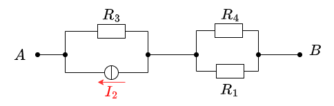
Aufgabe 4.5.2: open circuit voltage via superposition (exam task, approx. 12 % of a 60-minute exam, WS2020)

A circuit is given with the following parameters
$R_1=5 ~\Omega$
$U_1=2 ~\rm V$
$I_2=1 ~\rm A$
$R_3=20 ~\Omega$
$U_3=8 ~\rm V$
$R_4=10 ~\Omega$
Determine the open circuit voltage between A and B using the principle of superposition.
- What do the individual circuits look like, by which the effects of the individual sources can be calculated?
Which equivalent resistor must be used to replace a current or voltage source when calculating the individual effects? - Where are the open-circuit voltages applied when looking at the individual components?
(Voltage) source $U_1$
- substitute the current source $I_2$ with a short-circuit
- substitute the voltage source $U_3$ with an open circuit

The components can be moved in order to understand the circuit s bit better.

For the open circuit, no current is flowing through any resistor. Therefore, the effect is: $U_{AB,1} = U_1$
(current) source $I_2$
- substitute the voltage source $U_1$ with an open circuit
- substitute the voltage source $U_3$ with an open circuit

Also here, the components can be shifted for a better understanding:

Here, the current source $I_2$ creates a voltage drop $U_{AB_2}$ on the resistor $R_2$ : $U_{\rm AB,2} = - R_1 \cdot I_2$
(Voltage) source $U_3$
- substitute the voltage source $U_1$ with an open circuit
- substitute the current source $I_2$ with a short-circuit

Again, rearranging the circuit might help for an understanding:

In this case, between the unloaded outputs $\rm A$ and $\rm B$ there will be an unloaded voltage divider given by $R_3$ and $R_4$.
On $R_1$ there is no voltage drop since there is no current flow out of the unloaded outputs.
Therefore:
\begin{align*} U_{\rm AB,3} = \frac{R_4}{R_3 + R_4} \cdot U_3 \end{align*}
resulting voltage
\begin{align*} U_{\rm AB} &= U_1 - R_1 \cdot I_2 + \frac{R_4}{R_3 + R_4} \cdot U_3 \\ \end{align*}
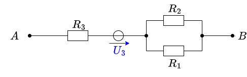
Exercise 4.5.3 -Variation: open circuit voltage via superposition (exam task, approx. 12 % of a 60-minute exam, WS2020)

A circuit is given with the following parameters
$R_1=5 ~\Omega$
$U_1=2 ~{\rm V}$
$I_2=1 ~{\rm A}$
$R_3=20 ~\Omega$
$U_3=8 ~{\rm V}$
$R_4=10 ~\Omega$
Determine the open circuit voltage between A and B using the principle of superposition.

\begin{align*} U_{\rm AB,1} = \frac{R_4}{R_1+R_4} U_1 = \frac{10~\Omega}{5~\Omega+10~\Omega} \cdot 2~{\rm V} = 1.33~{\rm V} \end{align*} Case 2: For this case is $U_1 = 0~{\rm V}$ and $U_3 = 0~{\rm V}$. The voltage is at $R_3$.
\begin{align*} U_{\rm AB,2} = R_3 I_2 = 20~\Omega \cdot 1~{\rm A} = 20~{\rm V} \end{align*} Case 3: For this case is $U_1 = 0~{\rm V}$ and $I_2 = 0~{\rm A}$. The voltage comes from the source $U_3$.
\begin{align*} U_{\rm AB,3} = 8~{\rm V} \end{align*} Superposition means adding the voltages of all three cases. \begin{align*} U_{\rm AB} = U_{\rm AB,1} + U_{\rm AB,2} + U_{\rm AB,3} = 1.33~{\rm V} + 20~{\rm V} + 8~{\rm V} \end{align*}
Exercise 4.5.4 - Variation: open circuit voltage via superposition (exam task, approx. 12 % of a 60-minute exam, WS2020)

A circuit is given with the following parameters
$I_1 = 2 ~{\rm A}$
$R_2 = 5 ~\Omega$
$R_3 = 20 ~\Omega$
$U_3 = 1 ~{\rm V}$
$R_4 = 10 ~\Omega$
$U_4 = 3 ~{\rm V}$
Determine the open circuit voltage between A and B using the principle of superposition.