Table of Contents
Block 08 — Two-terminal theory and transforms

Network analysis plays a central role in electrical engineering. It is so important because it can be used to simplify what at first sight appear to be complicated circuits and systems to such an extent that they can be understood and results derived from them.
In addition, networks also occur in other areas, for example, the momentum flux through a truss or the heat flux through individual hardware elements (figure 1, or an example for heat flow through electronics ). The concepts shown below can also be applied to these networks.
On the wiki page for network analysis the different methods are described very well in a compact way
8.0 Intro
8.0.1 Learning Objectives
- Define terminal and port; distinguish one-port (two-terminal) vs. two-port views; identify input/output variables $(U,I)$ at a port.
- Apply source transformations between a voltage source with series $R$ and a current source with parallel $R$ using $U_0=I_0\,R$; state validity conditions (linear, bilateral, time-invariant networks).
- Construct Thevenin and Norton equivalents seen at a port: find $U_{\rm oc}$, $I_{\rm sc}$, and $R_{\rm i}$ by deactivating sources; relate $U_{\rm Th}=U_{\rm oc}$, $R_{\rm Th}=R_{\rm i}$, $I_{\rm No}=I_{\rm sc}$.
- Use the superposition principle to compute branch currents/voltages in multi-source linear networks; outline the deactivate–solve–sum workflow.
- Combine transforms to reduce complex resistive networks to an unloaded / loaded divider and to size $R_{\rm L}$ for given performance goals (tie-in to Block 07 figures).
8.0.2 Preparation at Home
And again:
- Please read through the following chapter.
- Also here, there are some clips for more clarification under 'Embedded resources'.
For checking your understanding please do the following exercise:
- 4.5.3
8.0.3 90-minute plan
- Warm-up (8 min):
- Quick quiz on passive/active sign convention and $P=U\cdot I$ (from Block 07).
- Identify ports and choose measurement directions on 2–3 small circuits.
- Core concepts & derivations (58 min):
- (1) Source transformations ($U_0\leftrightarrow I_0$, shared $R$), permissible assumptions, and fast checks (10 min).
- (2) Thevenin/Norton construction at a chosen port: $U_{\rm oc}$, $I_{\rm sc}$, $R_{\rm i}$ (18 min).
- (3) Superposition method: deactivate sources, compute partial results, sum; worked DC example (15 min).
- Practice (20 min):
- Pair exercise set: reduce a 3-source network to Thevenin, then find $U_{\rm L}$, $I_{\rm L}$.
- Wrap-up (5 min):
- Summary table (when to use which method); minute paper: “One thing I can now do, one question I still have.”
8.0.4 Conceptual Overview
- Port thinking: Draw a virtual cut around the “rest of the world”. At that boundary (two terminals), everything inside looks like an equivalent linear source (Thevenin/Norton) to everything outside.
- Source transformations: A series source $(U_0, R)$ is equivalent to a parallel source $(I_0, R)$ if $U_0=I_0\,R$. Use them to simplify ladders and to expose a clean port.
- Thevenin/Norton from measurements:
- Open-circuit the load → measure/compute $U_{\rm oc}=U_{\rm Th}$.
- Short the load (only if safe/valid) → $I_{\rm sc}=I_{\rm No}$.
- Deactivate sources → compute the internal resistance $R_{\rm i}=R_{\rm Th}=R_{\rm No}$.
- Superposition (linear networks only): Voltages and currents add; powers do not. For each source: deactivate the others (ideal $U$-sources → short; ideal $I$-sources → open), solve the partial, then sum with signs.
- Choosing a method: Use source transforms for quick topology changes, Thevenin/Norton to isolate a load, and superposition when multiple sources block easy reduction.
8.1 Core content
8.1.1 Two-Terminal Theory / One-Port Theory

In order to understand the two-terminal theory / one-port theory, we first have to understand what a Terminal and port is.
So, have a look to figure 1:
- A terminal or pole is simply an (imaginary or real) connector. This is shown in the diagram by a filled circle on one wire, plus a semicircle on the other wire
- A port is given by two terminals
But, how could this help us in simplifying circuits?
Well: Usually, the voltage over or the current into one component or a group of component has to be found.
Now, it is practical, that
- you can substitue every passive linear part (= consisting only of resistors) by a single equivalent resistor.
- you can substitue every active linear part (= consisting of resistors and sources) by a single equivalent linear source.
A linear part is here a cirucit consisting of linear components. In general, ohmic resistors, sources, capacitors and inductors are linear - here, we only look onto resistors. (non-linear are most of the semiconductor components, like diodes).
So, what can we do? Once you search for a distinct voltage or current:
- Imagine a virtual cut around this part. You get a passive linear part and a active linear part.
- Calculate the single equivalent resistor and single equivalent linear source. You get an unloaded voltage divider.
- Calculate the voltage divider
Voilà, we have a way to find our desired voltage or current in a complicated circuitry.
Hint:
There is a trick to get the internal resistance of the source easily, so without continuous back-and-forth beween linear voltage source and linear current source:When one is only interested in the resistance of a complex circuit, do as follows:
- substitute every ideal source with its internal resistance (ideal voltage source → short circuit, ideal current source → unconnected).
- calculate the eqivalent resistance by means of series and parallel sub-circuits.
8.1.2 Superposition Principle
The superposition principle shall first be illustrated by some examples:
Example 1 - from an interview of a consulting company
Task: Three students are to fill a pool. If Alice has to fill it alone, she would need 2 days. Bob would need 3 days and Carol would need 4 days. How long would it take all three to fill a pool if they helped together?
The question sounds far off-topic at first but is directly related. The point is that to solve it, filling the pool is assumed to be linear. So Alice will fill $1 \over 2$, Bob $1 \over 3$, and Carol $1 \over 4$ of the pool per day. So on the first day, ${1 \over 2}+{1 \over 3}+{1 \over 4} = {{6 + 4 + 3} \over 12} = {13 \over 12}$ of the pool filled.
So the three of them need ${12 \over 13}$ of a day.
However, this solution path is only possible because in linear systems the partial results can be added.
Example 2 - Spring Force and Displacement

Task:A mechanical, linear spring is displaced due to masses $m_1$ and $m_2$ in the Earth's gravitational field (see figure 3). What is the magnitude of the deflection if both masses are attached simultaneously?
Again, a linear law is used here: \begin{align*} \vec{s}= f(\vec{F}) = - D \cdot \vec{F} \end{align*}
The (seemingly trivial) approach applies here: \begin{align*} \vec{s}_{1+2} = f(\vec{F_1} + \vec{F_2}) &= - D \cdot (\vec{F_1} + \vec{F_2}) \\ &= - D \cdot \vec{F_1} - D \cdot \vec{F_2} \\ &= f(\vec{F_1}) + f(\vec{F_2}) \\ &= \vec{s_1} + \vec{s_2} \end{align*}
Notice:
In a physical system in which effect and cause are linearly related, the effect of each cause can first be determined separately. The total effect is then the sum of the individual effects.For electrical engineering this principle was described by Hermann_von_Helmholtz:
The currents in the branches of a linear network are equal to the sum of the partial currents in the branches concerned caused by the individual sources.
Thus, in the superposition method, the current (or voltage) sought in a circuit with multiple sources can be viewed as a superposition of the resulting currents (or voltages) of the individual sources.
The “recipe” for the overlay is as follows:
- Choose the next source
x - Replace all ideal sources with their respective equivalent resistors:
- ideal voltage sources by short circuits
- ideal current sources by an open line
- Calculate the partial currents sought in the branches considered.
- Go to the next source
x=x+11), and to point 2, as long as the partial currents of all sources have not been calculated. - Add up the partial currents in the branches under consideration, observing the correct sign.
This procedure is explained again in more detail using examples in the two videos on the right.
Simple view of the superposition principle
A more complex example of the superposition method
Example
Fig. 4: example circuit with superposition 
8.2 Common Pitfalls
- Deactivating sources incorrectly: replacing an ideal voltage source with an open (instead of a short), or an ideal current source with a short (instead of an open).
- Superposing powers: only $u$ and $i$ superpose; $P$ does not. Compute powers after summing.
- Illegal short/open tests: shorting across an element that cannot be shorted (e.g., an ideal current source without care) or opening where it breaks circuit definitions.
- Sign/arrow mismatches: mixing passive/active sign conventions leads to wrong partial signs in superposition.
- Applying linear methods to non-linear/time-varying parts: Thevenin/Norton and superposition require linearity (and usually bilateral behavior).
- Ignoring loading: using the unloaded divider ratio $\dfrac{R_2}{R_1+R_2}$ while a finite $R_{\rm L}$ is attached → systematic voltage error.
8.3 Exercises
Longer Exercises
Exercise E4.5.1 Converting a bipolar signal to a unipolar signal (HARD, not from written test)
Imagine you want to develop a circuit that conditions a sensor signal so that it can be processed by a microcontroller. The sensor signal is in the range $U_{\rm sens} \in [-15...15~\rm V]$, and the microcontroller input can read values in the range $U_{\rm uC} \in [0...3.3~\rm V]$. The sensor can supply a maximum current of $I_{\rm sens, max}=1~\rm mA$. For the internal resistance of the microcontroller, input applies: $R_{\rm uC} \rightarrow \infty$
For conditioning, the input signal is to be fed via the series resistor $R_3$ to the center potential of a voltage divider $R_1 - R_2$ with $R_1$ to a supply voltage $U_{\rm s}$.
The following simulation shows roughly the situation. Be aware that the resistor and voltage values are not correct!
Questions:
1. Find the relationship between $R_1$, $R_2$, and $R_3$ using superposition.
- Determine suitable values for $R_1$, $R_2$, and $R_3$.
- What values for $R^0_1$, $R^0_2$, and $R^0_3$ from the BROKEN-LINK:E24 series LINK-BROKEN can be used to do this?
To make the calculation simpler, the resistors $R_3$ and $R_{\rm s}$ will be joined to $R_4 =R_3 +R_{\rm s}$.
Circuit 1 : only consider $U_{\rm S}$, ignore $U_{\rm I}$

\begin{align*} U_{\rm O}^{(1)} &= U_{\rm S} \cdot {{R_2||R_4}\over{R_1 + R_2||R_4}} = U_{\rm S} \cdot {{ {{R_2 R_4}\over{R_2 + R_4}} }\over{R_1 + {{R_2 R_4}\over{R_2 + R_4}} }} \\ &= U_{\rm S} \cdot {{ R_2 R_4 }\over{R_1 (R_2 + R_4)+ R_2 R_4 }} \\ &= U_{\rm S} \cdot {{ R_2 R_4 }\over{R_1 R_2 + R_1 R_4 + R_2 R_4 }} \\ \end{align*}
Circuit 2 : only consider $U_{\rm I}$, ignore $U_{\rm S}$

\begin{align*} U_{\rm O}^{(2)} &= U_{\rm I} \cdot {{R_1||R_2}\over{R_4 + R_1||R_2}} = U_{\rm I} \cdot {{ {{R_1 R_2}\over{R_1 + R_2}} }\over{R_4 + {{R_1 R_2}\over{R_1 + R_2}} }} \\ &= U_{\rm I} \cdot {{ R_1 R_2 }\over{R_4 (R_1 + R_2)+ R_1 R_2 }} \\ &= U_{\rm I} \cdot {{ R_1 R_2 }\over{R_4 R_1 + R_4 R_2+ R_1 R_2 }} \\ \end{align*}
Superposition: Let's sum it up!
These two intermediate voltages for the single sources have to be summed up as $U_{\rm O}= U_{\rm O}^{(1)} + U_{\rm O}^{(2)}$.
When deeper investigated, one can see that the denominator for both $U_{\rm O}^{(1)}$ and $U_{\rm O}^{(2)}$ is the same.
We can also simplify further when looking at often-used sub-terms (here: $R_2$)
\begin{align*} U_{\rm O} &= {{ 1 }\over{R_4 R_1 + R_4 R_2+ R_1 R_2 }} \cdot (U_{\rm S} \cdot R_2 R_4 + U_{\rm I} \cdot R_1 R_2 ) \\ U_{\rm O} \cdot (R_4 R_1 + R_4 R_2+ R_1 R_2 ) &= U_{\rm S} \cdot R_2 R_4 + U_{\rm I} \cdot R_1 R_2 \\ \\ U_{\rm O} \cdot ({{R_1 R_4}\over{R_2}} + R_4 + R_1 ) &= U_{\rm S} \cdot R_4 + U_{\rm I} \cdot R_1 \tag 1 \\ \end{align*}
The formula $(1)$ is the general formula to calculate the output voltage $U_{\rm O}$ for a changing input voltage $U_{\rm I}$, where the supply voltage $U_{\rm S}$ is constant.
Now, we can use the requested boundaries:
- For the minimum input voltage $U_{\rm I}= -15 ~\rm V$, the output voltage shall be $U_{\rm O} = 0 ~\rm V$
- For the maximum input voltage $U_{\rm I}= +15 ~\rm V$, the output voltage shall be $U_{\rm O} = 3.3 ~\rm V$
This leads to two situations:
Situation I : $U_{\rm I,min}= -15 ~\rm V$ shall create $U_{\rm O,min} = 0 ~\rm V$
We put $U_{\rm A} = 0 ~\rm V$ in the formula $(1)$ :
\begin{align*}
0 &= U_{\rm S} \cdot R_4 + U_{\rm I,min} \cdot R_1 \\
- U_{\rm I,min} \cdot R_1 &= U_{\rm S} \cdot R_4 \\
{{R_1}\over{R_4}} &=-{{U_{\rm S}}\over {U_{\rm I,min}}} = k_{14} \tag 2 \\
\end{align*}
So, with formula $(2)$, we already have a relation between $R_1$ and $R_4$. Yeah 😀
The next step is situation 2
Situation II : $U_{\rm I,max}= +15 ~\rm V$ shall create $U_{\rm O,max} = 3.3 ~\rm V$
We use formula $(2)$ to substitute $R_1 = k_{14} \cdot R_4 $ in formula $(1)$, and:
\begin{align*}
U_{\rm O,max} \cdot (k_{14}{{ R_4^2}\over{R_2}} + R_4 + k_{14} R_4 ) &= U_{\rm S} \cdot R_4 + U_{\rm I,max} \cdot k_{14} R_4 \\
U_{\rm O,max} \cdot (k_{14}{{ R_4 }\over{R_2}} + 1 + k_{14} ) &= U_{\rm S} + U_{\rm I,max} \cdot k_{14} \\
k_{14}{{ R_4 }\over{R_2}} + 1 + k_{14} &= {{U_{\rm S} + U_{\rm I,max} \cdot k_{14} }\over{ U_{\rm O,max} }} \\
k_{14}{{ R_4 }\over{R_2}} &= {{U_{\rm S} + U_{\rm I,max} \cdot k_{14} }\over{ U_{\rm O,max} }} - (1 + k_{14})\\
{{ R_4 }\over{R_2}} &= {{U_{\rm S} + U_{\rm I,max} \cdot k_{14} }\over{ k_{14} U_{\rm O,max} }} - {{1 + k_{14} }\over{k_{14}}} \tag 3 \\
\end{align*}
So, another relation for $R_4$ and $R_2$. 😀
So, to get values for the relations, we have to put in the values for the input and output voltage conditions. For $k_{14}$ we get by formula $(2)$: \begin{align*} k_{14} = {{R_1}\over{R_4}} =-{{5 ~\rm V}\over {-15 ~\rm V }} = {{1}\over{3}} \\ \end{align*}
This value $k_{14}$ we can use for formula $(3)$: \begin{align*} {{ R_4 }\over{R_2}} &= {{5 ~\rm V + 15 ~\rm V \cdot {{1}\over{3}} }\over{ 3.3 ~\rm V \cdot {{1}\over{3}} }} - {{1 + {{1}\over{3}} }\over{ {{1}\over{3}} }} \\ &= {{10}\over{1.1}} - 4 \\ k_{42} &\approx 5.09 \end{align*}
We could now - theoretically - arbitrarily choose one of the resistors, e.g., $R_2$, and then calculate the other two.
But we must consider another boundary, a boundary for $R_{\rm S}$. The maximum voltage and the maximum current are given for the sensor. By this, we can calculate $R_{\rm S}$: \begin{align*} R_{\rm S} &= {{ U_{\rm OC} }\over{ I_{\rm SC} }} = {{ U_{\rm S,max} }\over{ I_{\rm S,max} }} = {{ 15 ~\rm V }\over{ 1 ~\rm mA }} \\ &= 15 ~\rm k\Omega \end{align*}
Therefore, $R_4 = R_{\rm S} + R_3$ must be larger than this.
The sensor resistance is \begin{align*} R_S &= 15 {~\rm k\Omega}\\ \end{align*}
We can choose $R_3$ arbitrarily. Here I choose a nice value to get integer values for $R_3$ and $R_1$: \begin{align*} R_3 &= 45 {~\rm k\Omega}\\ R_1 &= {{1}\over{3}} (R_3 + 15 {~\rm k\Omega}) = 20 {~\rm k\Omega} \\ R_2 &= {{1}\over{5.09}}(R_3 + 15 {~\rm k\Omega}) = 11.8 {~\rm k\Omega} \end{align*}
Based on the E24 series, the following values are next to the calculated ones: \begin{align*} R_3^0 &= 43 {~\rm k\Omega}\\ R_1^0 &= {{1}\over{3}} (R_3 + 15 {~\rm k\Omega}) = 20 {~\rm k\Omega} \\ R_2^0 &= {{1}\over{5.09}}(R_3 + 15 {~\rm k\Omega}) = 12 {~\rm k\Omega} \end{align*}
2. Find the relationship between $R_1$, $R_2$, and $R_3$ by investigating Kirchhoff's nodal rule for the node where $R_1$, $R_2$, and $R_3$ are interconnected.
The potential of the node is $U_\rm O$. Therefore the currents are:
- the current $I_2$ over $R_2$ is flowing to ground: $I_2 = - {{U_\rm O}\over{R_2}} $
- the current $I_1$ over $R_1$ is coming from the supply voltage $U_{\rm S}$ to the nodal voltage $U_{\rm O}$: $I_1 = {{U_{\rm S} - U_{\rm O}}\over{R_1}}$
- the current $I_4$ over $R_4$ is coming from the input voltage $U_{\rm I}$ to the nodal voltage $U_{\rm O}$: $I_4 = {{U_{\rm I} - U_{\rm O}}\over{R_4}}$
This led to the formula based on the Kirchhoff's nodal rule:
\begin{align*} \Sigma I = 0 &= I_1 + I_2 + I_3 \\ 0 &= {{U_{\rm S} - U_{\rm O}}\over{R_1}} + {{U_{\rm I} - U_{\rm O}}\over{R_4}} - {{U_\rm O}\over{R_2}} \end{align*}
The formula can be rearranged, with all terms containing $ U_{\rm O}$ on the left side: \begin{align*} {{U_{\rm O}}\over{R_1}} + {{U_{\rm O}}\over{R_2}} + {{U_{\rm O}}\over{R_4}} &= {{U_{\rm S}}\over{R_1}} + {{U_{\rm I}}\over{R_4}} \\ U_{\rm O}\cdot \left( {{1}\over{R_1}} + {{1}\over{R_2}} + {{1}\over{R_4}} \right) &= {{U_{\rm S}}\over{R_1}} + {{U_{\rm I}}\over{R_4}} \\ \end{align*}
Both sides can be multiplied by $\cdot R_1$, $\cdot R_2$, $\cdot R_4$ - in order to get rid of the fractions : \begin{align*} U_{\rm O}\cdot \left( {{R_1 R_2 R_4 }\over{R_1}} + {{R_1 R_2 R_4 }\over{R_2}} + {{R_1 R_2 R_4 }\over{R_4}} \right) &= R_1 R_2 R_4 \cdot {{U_{\rm S}}\over{R_1}} + R_1 R_2 R_4 \cdot {{U_{\rm I}}\over{R_4}} \\ U_{\rm O}\cdot \left( R_2 R_4 + R_1 R_4 + R_1 R_2 \right) &= R_2 R_4 \cdot U_{\rm S} + R_1 R_2 \cdot U_{\rm I} \\ U_{\rm O} &= {{R_2}\over{R_2 R_4 + R_1 R_4 + R_1 R_2 }} \left( R_4 \cdot U_{\rm S} + R_1 \cdot U_{\rm I} \right)\\ \end{align*}
The last formula was just the result we also got by the superposition but by more thinking.
So, sometimes there is an easier way…
- Unluckily, there is no simple way to know before, what way is the easiest.
- Luckily, all ways lead to the correct result.
3. What is the input resistance $R_{\rm in}(R_1, R_2, R_3)$ of the circuit (viewed from the sensor)?
\begin{align*} R_{\rm in}(R_1, R_2, R_3) &= R_3 + R_1 || R_2 \\ &= R_3 + {{R_1 R_2}\over{R_1 + R_2}} \end{align*}
4. What is the minimum allowed input resistance ($R_{\rm in, min}(R_1, R_2, R_3)$) for the sensor to still deliver current?
\begin{align*} R_{\rm in, min} &= {{U_{\rm sense}}\over{I_{\rm sense, max}}} \\ &= \rm {{15 V}\over{1 mA}} \\ &= 15 k\Omega \\ \end{align*}
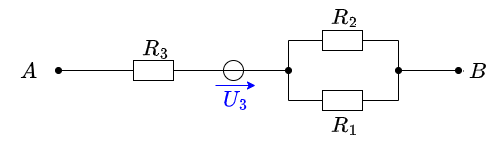
Aufgabe 4.5.2: open circuit voltage via superposition (exam task, approx. 12 % of a 60-minute exam, WS2020)

A circuit is given with the following parameters
$R_1=5 ~\Omega$
$U_1=2 ~\rm V$
$I_2=1 ~\rm A$
$R_3=20 ~\Omega$
$U_3=8 ~\rm V$
$R_4=10 ~\Omega$
Determine the open circuit voltage between A and B using the principle of superposition.
- What do the individual circuits look like, by which the effects of the individual sources can be calculated?
Which equivalent resistor must be used to replace a current or voltage source when calculating the individual effects? - Where are the open-circuit voltages applied when looking at the individual components?
(Voltage) source $U_1$
- substitute the current source $I_2$ with a short-circuit
- substitute the voltage source $U_3$ with an open circuit

The components can be moved in order to understand the circuit s bit better.

For the open circuit, no current is flowing through any resistor. Therefore, the effect is: $U_{AB,1} = U_1$
(current) source $I_2$
- substitute the voltage source $U_1$ with an open circuit
- substitute the voltage source $U_3$ with an open circuit

Also here, the components can be shifted for a better understanding:

Here, the current source $I_2$ creates a voltage drop $U_{AB_2}$ on the resistor $R_2$ : $U_{\rm AB,2} = - R_1 \cdot I_2$
(Voltage) source $U_3$
- substitute the voltage source $U_1$ with an open circuit
- substitute the current source $I_2$ with a short-circuit

Again, rearranging the circuit might help for an understanding:

In this case, between the unloaded outputs $\rm A$ and $\rm B$ there will be an unloaded voltage divider given by $R_3$ and $R_4$. On $R_1$ there is no voltage drop since there is no current flow out of the unloaded outputs.
Therefore:
\begin{align*} U_{\rm AB,3} = \frac{R_4}{R_3 + R_4} \cdot U_3 \end{align*}
resulting voltage
\begin{align*} U_{\rm AB} &= U_1 - R_1 \cdot I_2 + \frac{R_4}{R_3 + R_4} \cdot U_3 \\ \end{align*}
Exercise 4.5.3 -Variation: open circuit voltage via superposition (exam task, approx. 12 % of a 60-minute exam, WS2020)

A circuit is given with the following parameters
$R_1=5 ~\Omega$
$U_1=2 ~{\rm V}$
$I_2=1 ~{\rm A}$
$R_3=20 ~\Omega$
$U_3=8 ~{\rm V}$
$R_4=10 ~\Omega$
Determine the open circuit voltage between A and B using the principle of superposition.

\begin{align*} U_{\rm AB,1} = \frac{R_4}{R_1+R_4} U_1 = \frac{10~\Omega}{5~\Omega+10~\Omega} \cdot 2~{\rm V} = 1.33~{\rm V} \end{align*} Case 2: For this case is $U_1 = 0~{\rm V}$ and $U_3 = 0~{\rm V}$. The voltage is at $R_3$.
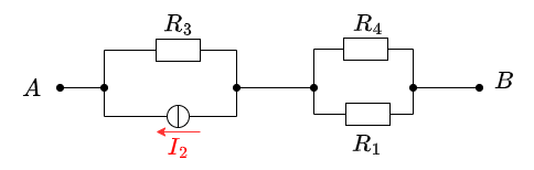
\begin{align*} U_{\rm AB,2} = R_3 I_2 = 20~\Omega \cdot 1~{\rm A} = 20~{\rm V} \end{align*} Case 3: For this case is $U_1 = 0~{\rm V}$ and $I_2 = 0~{\rm A}$. The voltage comes from the source $U_3$.
\begin{align*} U_{\rm AB,3} = 8~{\rm V} \end{align*} Superposition means adding the voltages of all three cases. \begin{align*} U_{\rm AB} = U_{\rm AB,1} + U_{\rm AB,2} + U_{\rm AB,3} = 1.33~{\rm V} + 20~{\rm V} + 8~{\rm V} \end{align*}
Exercise 4.5.4 - Variation: open circuit voltage via superposition (exam task, approx. 12 % of a 60-minute exam, WS2020)

A circuit is given with the following parameters
$I_1 = 2 ~{\rm A}$
$R_2 = 5 ~\Omega$
$R_3 = 20 ~\Omega$
$U_3 = 1 ~{\rm V}$
$R_4 = 10 ~\Omega$
$U_4 = 3 ~{\rm V}$
Determine the open circuit voltage between A and B using the principle of superposition.
Embedded resources
Introduction to Superposition Method (starting from 34:24, Befor there are other methods not covered here)