This is an old revision of the document!
3. Combinatorical Logic
introductional example
The combinatorial logic shown in <impref pic1> enables to output distinct logic values for eacht logic input. When you change the input nibble you can see that the the correct number appears on the 7-segment-display. By clicking onto the bits of the input nibble, you can change the number.
Tasks:
- Which output $Y_0$ … $Y_6$ is generated from the input nibble
1000? Which from1001? - Is the output only depending on the input? Is there a dependance on the histroy?
3.1 Combinatorical Circuit
Up to now, we looked onto simple logic circuits. Thes are relatively easy to analyze and synthesize (=develop). The main question in this chapter is: how can we set up and optimize logic circuits?
In the following we have a look onto combinatorical circuits. These are generally logic circuits with
- $n$ inputs $X_0$, $X_1$, … $X_{n-1}$
- $m$ outputs $Y_0$, $Y_1$, … $Y_{m-1}$
- no “memory”, that is: a given set of input bits results in a distinct output
They can be description by
- truth table
- boolean formula
- hardware description language
The ladder one is not in the focus of this course.
The applications range:
- (simple) half/full adder
- digital comparators (logic circuit to compare 2 values)
- Multiplexer / demultiplexer
- Arithmetic logic units in microcontrollers and processors
- much more
3.1.1 Example
In order to understand the synthesis of a combinatoric logic we will follow a step-by-step example for this chapter.
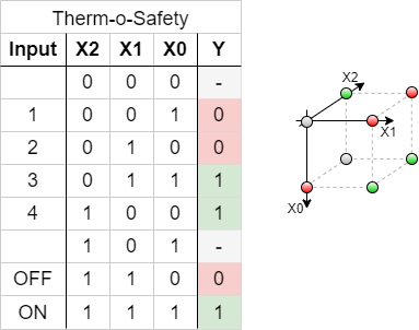
Imagine you are working for a company called “mechatronics and robotics”. One costumer wants to have an intelligent switch as input device connected to a microcontroller for controlling an oven. For this project “Therm-o-Safety” he needs a combinatoric logic:
- The intelligent switch has 4 user selectable positions: $1$, $2$, $3$, $4$
- Additionally there are 2 non-selectable positions for the case of failure.
- The output $Y=1$ will activate a temperature monitoring.
- The temperature monitoring has to be active for $3$ and $4$ and in case of a major failure. A major failure is for example, when the switch position is unclear. In this case the input of the combinatorial circuit is “ON”.
- There are no other cases of inputs.
This requirements are put into a truth table:
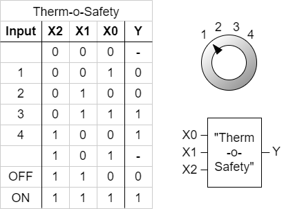
figure 2 shows one implementation of this requirements. The inputs 001 … 011 represent the inputs $1$…$4$. The cases of failure are coded with 110 and 111.
The output $Y$ is activated as requested. For the two combinations 000 and 101 there is no output value defined. Depending on the requierements for a project these shall either better be 0 or 1 or the output of these does not matter. We had this “does not matter” before: the technical term is “I don't care”, and it is written as a - or a x.
By this, we have done the first step in order to syntesize the requested logic.
3.1.2 Sum of Products
Now, we want to investigate some of the input combinations (= lines in the truth table). At first, we have a look onto the input combination 011, where the output has to be $Y=1$.
If this input combination would be the only one for the output of $Y=1$, the following could be stated:
“$Y=1$ (only) when the $X_0$ is $1$ AND $X_1$ is $1$ AND $X_2$ is $0$ ”. It can also be re-arranged to:
“$Y=1$ (only) when the $X_0$ is $1$ AND $X_1$ is $1$ AND $X_2$ is not $1$ ”.
This statement is similar to $X_0 \cdot X_1 \cdot \overline{X_2}$. The used conjuntion resuts only in $1$, when all inputs are $1$. The negation of $X_2$ takes account of the fact, that $X_2$ has to be $0$.
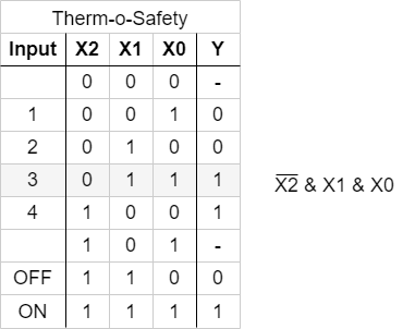
figure 3 shows the boolean expression for ths combination. In figure 4, this boolean expression is converted into a struction with logic gates.
With the same idea in mind, we can have a look for the other combinations resulting in $Y=1$. These are the combinations 100 and 111:
- For
100The statement would be: “$Y=1$ (only) when the $X_0$ is $0$ AND $X_1$ is $0$ AND $X_2$ is $1$”. Similary to the combination above this leads to: $\overline{X_0} \cdot \overline{X_1} \cdot {X_2}$. - For
111, the boolean expression is ${X_0} \cdot {X_1} \cdot {X_2}$.
Note!
- Each row in a truth table (=one distinct combination) can be represented by a minterm or maxterm
- A minterm is the conjunction (AND'ing) of all inputs, where unter certain instances a negation have to be used
- In a minterm an input variable with
0has to be negated, in order to use it as an input for the AND.
e.g. $X_0 = 0$ AND $X_1 = 1$$ \quad \rightarrow \quad \overline{X_0} \cdot X_1$ - A minterm results in a output of
1
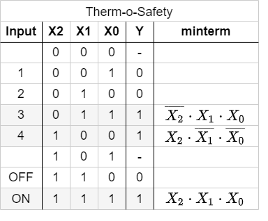
In figure 5 all minterms for $Y=1$ are shown. The figure 6 depicts all the logic circuits for the three minterms. These lead to the outputs $Y'$, $Y''$, and $Y'''$.
For the final step we have to combine the single results for the minterms. The output has to be $1$ when at least one of the minterms is $1$. Therefore, the minterms have to be connected disjunctive:
\begin{align*} Y &= & Y' & \quad + & Y'' & \quad + & Y''' \\ Y &= & (X_0 \cdot X_1 \cdot \overline{X_2}) & \quad + & (\overline{X_0} \cdot \overline{X_1} \cdot {X_2}) & \quad + & ({X_0} \cdot {X_1} \cdot {X_2}) \\ \end{align*}
This leads to the logic circuit shown in figure 7. Here, you can input the different combinations by clicking onto the bits of the input nibble.
Note!
- The disjunction of the minterms is called sum of products, SoP, disjunctive normal form or DNF.
- When all inputs are used in each of the minterms the normal form is called full disjunctive normal form
- When snytesizing a logic circuit by sum of products, all 'don't care' terms outputing $0$.
We have seen, that the sum of products is one tool to derive a logic circuit based on a truth table. Alternatively it is also possible to insert an intermediate step, where the logic formula is simplified.
In the following one possible optimization is shown:
\begin{align*} Y &= & (X_0 \cdot X_1 \cdot \overline{X_2}) & \quad + & (\overline{X_0} \cdot \overline{X_1} \cdot {X_2}) & \quad + & ({X_0} \cdot {X_1} \cdot {X_2}) & \quad | \text{associative law} \\ Y &= & (\overline{X_0} \cdot \overline{X_1} \cdot {X_2}) & \quad + & (X_0 \cdot X_1 \cdot \overline{X_2}) & \quad + & ({X_0} \cdot {X_1} \cdot {X_2}) & \quad | \text{associative law } \\ Y &= & (\overline{X_0} \cdot \overline{X_1} \cdot {X_2}) & \quad + & ((X_0 \cdot X_1) \cdot \overline{X_2}) & \quad + & (({X_0} \cdot {X_1}) \cdot {X_2}) & \quad | \text{distributive law } \\ Y &= & (\overline{X_0} \cdot \overline{X_1} \cdot {X_2}) & \quad + & ((X_0 \cdot X_1) \cdot (\overline{X_2} + {X_2})) & & & \quad | \text{complementary element} \\ Y &= & (\overline{X_0} \cdot \overline{X_1} \cdot {X_2}) & \quad + & (X_0 \cdot X_1) \\ \end{align*}
3.1.3 Product of Sums
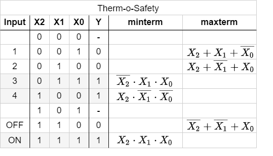
In the sub-chapter before we had a look onto the combinations which generates an output of $Y=1$ by means of the AND operator. Now we are investigating the combinations with $Y=0$. Therefore, we need an operator, which results in $0$ for only on distinct combination.
The first combination to look for is 001.
If this input combination would be the only one for the output of $Y=0$, the following could be stated:
“$Y=0$ (only) when the $X_0$ is $1$ AND $X_1$ is $0$ AND $X_2$ is $0$ ”.
With having the duality in mind (see cpt. The Set of Rules) the opposite is also true:
“$Y=1$ when $X_0$ is $0$ OR $X_1$ is $1$ OR $X_2$ is $1$ ”
This is the same like: $\overline{X_0} + X_1 + X_2$
The booleand operator we need hiere is the OR-operator.
Simmilarly, the combinations 010 und 110 can be transformed. Keep in mind, that this time we are looking for a formula with results in $0$ only for the given one distinct combination.
Note!
- A maxterm is the disjunction (OR'ing) of all inputs, where unter certain instances a negation have to be used.
- In a maxterm an input variable with
1has to be negated, in order to use it as an input for the OR. - A maxterm results in a output of
0
The figure 8 shows all the maxterms for the Therm-o-Safety example.
The formulas of figure 8 can again be transformed into gate circiuts (figure 9). Here, only for the inputs '001', '010', '110' one of the outputs $Y'$, $Y''$ or $Y'''$ is $0$.
When these intermediate outputs $Y'$, $Y''$, $Y'''$ are used as an input for an AND-gate the resultin output will get $0$ when at least one of the intermediate outputs are $0$. This results in another way to synthesize the Therm-o-Safety (see figure 10)
Also the products of sum can be simplified:
\begin{align*} Y &= & (\overline{X_0} + X_1 + X_2) & \quad \cdot & ({X_0} + \overline{X_1} + X_2) & \quad \cdot & (\overline{X_0} + \overline{X_1} + X_2) \\ &= & ... \\ Y &= & (\overline{X_0} + X_1 + X_2) & \quad \cdot & (\overline{X_0} + \overline{X_1}) \\ \end{align*}
This result $Y$ by the sum of products is different compared to the result in product of sums:
- product of sums: $Y = (\overline{X_0} \cdot \overline{X_1} \cdot {X_2}) + (X_0 \cdot X_1)$
- sum of products: $Y = (\overline{X_0} + X_1 + X_2) \cdot (\overline{X_0} + \overline{X_1})$
In this case these resuls cannot be transformed into each other with the means of boolean rules.
Note!
- The disjunction of the maxterms is called products of sum, PoS, conjunctive normal form or CNF.
- When all inputs are used in each of the minterms the normal form is called full conjunctive normal form
- When snytesizing a logic circuit by sum of procucts, all 'don't care' terms outputing $1$
- The products of sum is the DeMorgan dual of the sum of products if there are no don't care terms. Otherwise the resuls cannot be transformed into each other with the means of boolean rules.
3.2 Karnaugh Map
3.2.1 Introduction with the two dimensional Map
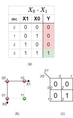
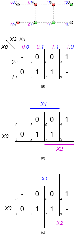
For a simple introduction we take one step back and look onto a simple example. The formula $Y(X_1, X_0) = X_0 \cdot X_1$ combines two variables. Therefore, it has two dimensions. In figure 11 (a) the truth table of this is shown. The most left column shows the decimal interpretation of the binary numeral given by $X_1$, $X_0$ (e.g. $(X_1=1, X_0=0) \rightarrow 10_2=2_{10}$).
The given logic expression can also be interpreted in in a coordinate system, with the following conditions:
- There are be only two coordinates on each axis possible:
0and1. - There are as much axis as variables given in the logic: For the example we have two variables $X_0$ and $X_0$. These are spanning a two dimensional system.
- On the possible positions, the results $Y$ have to be shown.
In the following pictures of this representation the values are shown as:
- green dot, when the result is
1 - red dot, when the result is
0 - grey dot, when the result is
don't care
For the given example the coordinate system shows four possible positions: This are the edges of a square (figure 11 (b)).
We will in the future write this as in figure 11 (c). This diagram is also called karnaugh map (often called k-map or KV map). In the shown Karnaugh map the coordinate $X_0$ is shown vertically and $X_1$ horizontally. Similar to the coordinate system the upper left cell is for $X_1=0$ and $X_0=0$. The upper right cell is for $X_1=1$ and $X_0=0$, the lower right one for $X_1=1$ and $X_0=1$. In each cell the result $Y(X_1,X_0)$ is shown as large number - similar to the color code in the coordinate system. The small number is the decimal representation of the number given by $X_1$ and $X_0$. This index is often not explicitly shown in the Karnaugh map, but simplifies the fill-in of the map and helps for the start.
The karnaugh map will help us in the following to find simplifications of more complex logic expressions.
3.2.2 The three dimensional Karnaugh Map
In this subchapter we will have a look onto our example of the therm-o-safety. For this example we found two possible gate logics which can produce the required output. We have also seen, that optimizing the terms (i.e. the min- or maxterms) is often possible. But we do not know how we can find the optimum implementation.
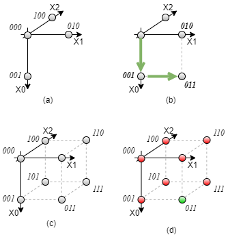
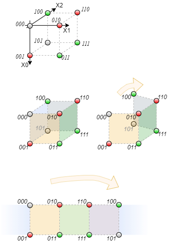
For this, we try to interpret the inputs of our example again as dimensions in a multidimensional space. The three input variables $X_0$, $X_1$, $X_2$ span a 3-dimensional space. The point 000 is the origin of this space. The three combinations 001, 010, 100 are onto the $X_0$-, $X_1$-, and $X_2$-axis, respectively (see figure 12 (a)). The other combinations can be reached by adding these axis values together (see figure 12 (b)+(c)). This is similar to the situation of a two dimensional or three dimensional vector. Three inputs result in this representation in the edges of a cube.
In the figure 12 (d) the situation $X_0=1$, $X_1=1$, $X_2=0$ is shown.
There is also an alternative way to look onto this representation:
- The formula $Y=1$ (independent from inputs $X_0...X_{n-1}$) lead to all positions are
1 - A single input equal
1( $Y:\, X_0=1$, independent from all other inputs, i.e. all others aredon't care) lead in the three dimansional example to the edges of a side surface of the cube.
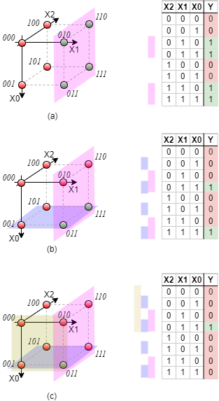
In out example $\color{violet}{X_1=1}$ lead to the situation shown in figure 13 (a). When investigating the shown green dots010,011,110,111it is visible that the middle value (= the value for $X_1$) is the same.
Generally: A single input equal1(independent from all other inputs) lead to a structure one dimension smaller than the number of inputs (In our example: 3 inputs $\rightarrow$ two dimensional structure = surface). - Multiple given inputs equal
1lead to smaller structures correspondingly. In our example: $\color{blue}{X_0=1}$ and $\color{violet}{X_1=1}$ ($=\color{blue}{X_0}\cdot \color{violet}{X_1}$) result in the two edges on a corner of the cube (figure 13 (b)). For this coordinates (011,111) the last two values are the same. - A minterm (=
1as an output) in our example is given by the intersection of all surfaces for the individual dimensions. In our example:$\color{blue}{X_0=1}$ and $\color{violet}{X_1=1}$ and $\color{brown}{X_2=0}$ ($=\color{blue}{X_0}\cdot \color{violet}{X_1}\cdot \color{brown}{\overline{X_2} }$) result in the two edges on a corner of the cube (figure 13 (c))
On the right side of figure 13 also the truth table is shown. There, the combinations for each side surfaces of the cube is marked with the corresponding color.
With this representation in mind, we can simplify other representations much more simplier.
One example for this would be to represent the formula: $Y= X_0 \cdot X_1 \cdot \overline{X_2} + X_2 \cdot X_1 + X_0 \cdot X_1 $. By drawing this into the cube one will see that it represents only a side surface of the cube. It can be simplified into $Y=X_1$.
We can also try to interpret our Therm-o-Safety truth table. The figure 14 shows the corresponding cube. The problem here is, that it is a bit unhandy to reduce a three dimansional cube onto a flat monitor or a paper. It will also get more stressfull for higher dimensions.
Therefore, we try to find a better way to sketch the coordinates, before we simplify our Therm-o-Safety. For the three dimensional Karnaugh map it is a good idea “unwrap” the cube. This can be done as shown in figure 15.
Out of the flattened cube we can derive the three dimensional Karnaugh map (see figure 16). Generally, there are different ways to show the Karnaugh map.
- One way is to show the variable names of the dimensions in the corner. Be aware, that the order of the numbers in horizontal direction is
0,0,0,1,1,1,1,0and not in ascending order! - In other ways the columns / rows related to the dimension are marked with lines. In this represenation only the
TRUE(=1) position of the coordinate is highlighted.
In figure 16 the dimensions are additionally marked with colors.
In the following chapters mainly the visualisation shown in figure 16 (b) is used.
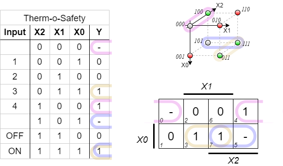
With this representation we can now try to read out the logic terms for the Therm-o-Safety from its Karnaugh map. figure 17 shows the neighbouring combinations:
- In light brown the group (
011+111) resp. position 3 and position 7 is shown. This can be simplified into $X_0 \cdot X_1$ - In light blue the group (
101+111) resp. position 5 and position 7 is shown. This can be simplified into $X_0 \cdot X_2$. This group seems not to be needed, since111is already in the light brown group. - In light violet the group (
000+100) resp. position 0 and position 4 is shown. This can be simplified into $\overline{X_0} \cdot \overline{X_1}$
The first two groups are also neighbouring cells in the Karnaugh map. For the last one we have to keep in mind, that we had to cut the surface of the cube in order to flatten it. Therefore, this cells are also neighbouring. These leads to the conclusion, that the borders of the Karnaugh map are connected to the opposite borders!
For our example the result would be: (light brown the group) + (light violet the group) $= X_0 \cdot X_1 + \overline{X_0} \cdot \overline{X_1}$
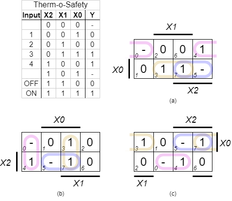
We also have to remember, that there are multiple permutations to show exacly the same logic assignment. This can be interpreted as other ways to unwrap the cube. The figure 18 shows the variant from before at (a). In image (b) the coordinates are mixed ($X_0 \rightarrow X_1$, $X_1 \rightarrow X_2$, $X_2 \rightarrow X_0$). In the image (c) the position of the origin is not on the upper left corner anymore.
Independent from the permutation, the grouped cells are always neighbouring each other.
Note!
- The Karnaugh map is an alternative way to represent a logic relation.
- There are possible grouping in order to simplify the logic.
- We need to take care of whether a group is needed or not. (will be done in chapter 3.3)
3.2.3 Four Dimensional Karnaugh Map
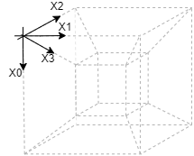
For the four dimensional Karnaugh map the situation becomes in the classical coordinate system more complicated. The respective object would be a four-dimensional hypercube (see figure 19). This is hard to print in a two dimensional layout like on a website or on a page. Here, a four dimensional Karnaugh map might be a good representation.
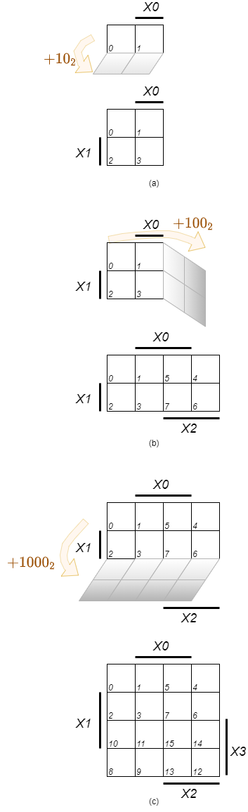
In order to create a four dimensional Karnaugh map, we look at first how the two and three dimensional Karnaugh map can be derived. The figure 20 (a) shows, that the two dimensional Karnaugh map can be created from a one dimensional one by folding the table on the x-axis and adding $10_2$ to all values. The additional line is marked with the new dimension $X_1$.
The three dimensional one is created by folding the table on the y-axis and adding $100_2$ to all values. The additional line is marked with the new dimension $X_2$ (figure 20 (b) ). Be aware, that the $X_0$ marking now has to be extended - it is also folded to the right.
The four dimensional one is created by folding the table again on the x-axis and adding $100_2$ to all values. The additional line is marked with the new dimension $X_2$ (figure 20 (c) ).
By this we can visually derive the four dimensional Karnaough map.
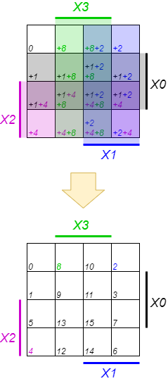
Again, there are alternative ways to show the Karnaugh map. To get the index of each cell one can easily add up the values of the dimension $X_0 ... X_3$. This is shown on an example in figure 21.
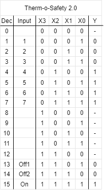
For getting used to the four dimensional Karnaugh map, we expand our Therm-o-Safety: Instead of four user selectable levels for oven, the version 2.0 will have seven. The temperature monitoring ($Y=1$) has to be active starting with level $4$. Additionally, the Therm-o-Safety 2.0 has three non-selectable positions for the case of failure, where the last one needs active temperature monitoring. Some of the combinations (0000, 1000, 1001, 1010, 1011, 1100) are not needed.
The truth table of the new Therm-o-Safety 2.0 is shown in figure 19
Now we can fill the Karnaugh map:
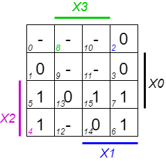
Disjunctive Form
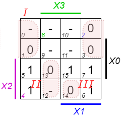
The Karnaugh map can now be used to either get the disjunctive form (= sum of products) when looking onto the groups of $1$s, or the conjunctive form (= product of sums) out of the groups of $0$s. We will at first look onto the disjunctive form. There are multiple way to group the minterms. One is shown here:
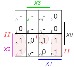
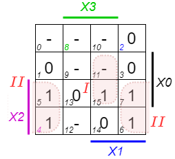
The group $I$ in figure 24 can be expanded, since there are don't care states nearby:
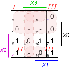
This can be transformed back into a formula. We can derive the boolean terms from the Karnaugh map with the folloring steps (see figure 26):
- Investigate each single group individually.
- For the sum of products each group has to be the product (AND-combination) of the inputs / coordinates.
- Then the formula can be derived as the sum of products…
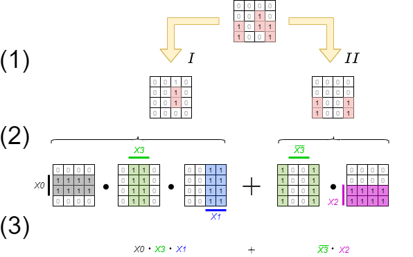
The given groups are created as a product as following:
- group $I$: all of this minterms are in the columns of $\color{green}{X_3}$. They are also all in the columns of $\color{blue}{X_1}$ and in the rows of $X_0$. This leads to $X_0 \cdot \color{green}{X_3} \cdot \color{blue}{X_1}$
- group $II$: all of this minterms are in the columns of $\color{green}{\overline{X_3}}$. They are also all in the rows of $\color{magenta}{X_2}$. This leads to $\color{green}{\overline{X_3}} \cdot \color{magenta}{X_2}$
Out of this groups we can get the full formula by disjunctive combination: \begin{align*} Y &= X_0 \cdot \color{green}{X_3} \cdot \color{blue}{X_1} + \color{green}{\overline{X_3}} \cdot \color{magenta}{X_2} \end{align*}
Conjunctive Form
Similarily we look onto the conjunctive form. Here we have to find groups of $0$s. One way of grouping the maxterms is shown here:
The optimization would be:
Also here, we can derive the boolean terms from the Karnaugh map with the folloring steps (see figure 29):
- Investigate each single group individually.
- For the products of sum each group has to be the sum (OR-combination) of the inputs / coordinates.
Be aware, that for the OR-combination we get the groups of $0$s as “rest” of not marked cells! - In the end the formula can again be derived, now as the product of sums.
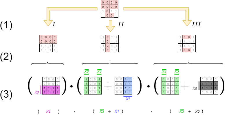
\begin{align*} Y &= ( \color{magenta}{X_2}) \cdot( \color{green}{\overline{X_3}} + \color{blue}{X_1}) \cdot( \color{green}{\overline{X_3}} + {X_0}) \end{align*}
Beyond the maxterms this formula can be optimized to
\begin{align*} Y &= \color{magenta}{X_2} \cdot( \color{green}{\overline{X_3}} + (\color{blue}{X_1} \cdot {X_0}) ) \end{align*}
When comparing the disjunctive solution ($X_3 \cdot X_1 \cdot X_0 + \cdot \overline{X_3} \cdot X_2 $) with the conjunctive one ($X_2 \cdot X_1 \cdot X_0 + \cdot \overline{X_3} \cdot X_2 $) we see, that these are definitely different. The given truth table had don't care states. This can be taken as $0$s or $1$s - and therefore combined in groups of $0$s or groups of $1$s.
3.2.4 Rules for the Karnaugh map
We saw, that with the Karnaugh map we can analyze logic combinations much better. But to use this tool right we have first to look onto some definitions.
Allowed Groups
As we have seen, the groups in the Karnaugh map are created by the combination of the inputs. By this only distinct groups are allowed. These can only have $2^{n-1}$ cells for $n$ inputs (= dimensions).
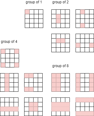
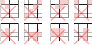
For a four dimensional Karnaugh map only the following groups are possible:
- groups of 1: Derived from 4 inputs, e.g. $X_3 \cdot \overline{X_2} \cdot \overline{X_1} \cdot \overline{X_0}$
- groups of 2: Derived from 3 inputs, e.g. $ \overline{X_3} \cdot {X_1} \cdot \overline{X_0}$
- groups of 4: Derived from 2 inputs, e.g. ${X_2} \cdot {X_0}$
- groups of 8: Derived from 1 inputs, e.g. $\overline{X_1} $
Exercise 3.1.x Further Querstions
- compare the results with the output given here (the output $y$ can be changed by clicking onto it)