This is an old revision of the document!
6. Sequential Logic
“I Know What You Did Last Cycle”
6.1 First Terminology
The most important term is the word state But what is a state? It is a unique situation, where the possible next steps (= possible next states), the inner behavior or the outputs are distinguishable from other situations. Here some practical examples:
- being happy or being sad, are two different states, since the inner behavior is different (this least often also to a different output). Similarly, an empty memory (or harddrive) is in a different state compared to an compared to a full one. Even a fresh deleted one is distingisable, since deletion
Sequential logic is used to describe logic cicruits which show internal states (“stateful”), and therefore have at least one memory element (= flip-flop).
The following terminology is used in the upcoming explanations:
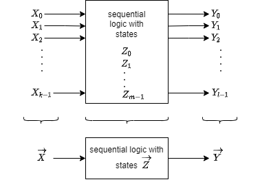
- The input vector $\vec{X}$ represents the $k$ inputs $X_0 ... X_{k-1}$
- The output vector $\vec{Y}$ represents the $l$ outputs $Y_0 ... Y_{l-1}$
- The state vector $\vec{Z}$ represents the $m$ inputs $Z_0 ... Z_{m-1}$
- The sign $(n)$ or $n$ marking the current point in time and therefore e.g. the current state $Z_0(n)$
- The sign $(n+1)$ or $n+1$ marking the next upcomming point in time and therefore e.g. the next state $Z_0(n+1)$
- Sequential logic circuits are also called Finite State Machines (FSM) or sometimes also shortened to “state machine”
The figure 12 shows the different terms in an abstract diagram. The “current” output values are here the values, which are shown after the delay time of the gates (about some nanoseconds).
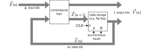
The principle interior of the blackbox in figure 12 was already shown in one practical application in the previous chapter: We saw, that we need the combination of an combinatorial logic and some storage components. Additionally, both have to be connected by feeding back some of the outputs back to the combinatorial logic. The output bits $\vec{Y}$ can result either from the combinatorial logic or the flip-flops. This is shown in figure 13.
Exercise 6.1.3.1 Example of a State Machine
figure 1 depicts a state machine.
- What happens, when $X$ is changed? On which edge the change is triggered?
- Write down how many components each vector $\vec{X}$ and $\vec{Y}$ has.
- How many bits (= flip flops) might the state vector $\vec{Z}$ need?
One simple example of a sequential logic is shown in figure 4. There, the combnatorial logic is explicitely shown. Depending on the input $X$ the output $\vec{Y}$ shows an up-counting 2-bit value counting $0 \rightarrow 1 \rightarrow 2 \rightarrow 3 \rightarrow 0 \rightarrow ...$. This is a simple state machine which will be used in the net chapters
6.2 Classical State Machine Types
The up-counter in the previous sub-chapter was able to count from $0$ to $3$. But what can we do in order to count differently, like $ 7, 6, 1, 5$? In order to understand this, a simplier situation will be investigated. So, let's look how one can create a up-counter counting $1, 2, 3, 4$.
6.2.1 Moore Machine
The first idea might be to use what we already have: an up-counter, which faciliate 2 flip-flops in order to result into 2-bit output. The wanted new state machine needs 3 bits for the output, since the binary representation of our outputs are $%001$,$%010$,$%011$,$%100$.
An simple idea is to take the 2-bit up-counter and add an combinatorial logic in behind. This logic shall convert the 2-bit up-counter output $%00$ into $%001$, the $%01$ into $%010$, $%10$ into $%011$ and $%11$ into $%101$. This can be logic can be created by:
- writing down the truth table
- putting the values into a Karnaugh map
- extracting the formula with view onto the implicants
- generating the circuit with gates
When this is done, the result looks like figure 5
This resembles a so called Moore Machine
Note!
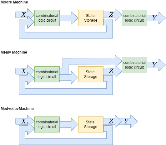
A state machine is a Moore Machine, when the output values $\vec{Y}$ depends only on the state values $\vec{Z}$. For this the moore machine uses two combinatorial circuits:
- The input circuit, which process the input values $\vec{X}(n+1)$ and the state values $\vec{Z}(n)$ (of the previous step) in such a way that the new states $\vec{Z}(n+1)$ are generated.
- The output circuit, which transform the state values $\vec{Z}(n)$ into the output values $\vec{Y}(n)$.
The properties of a moore machine are:
- The number of flip-flops is only given by number of states $m$.
- The output only changes when an edge on the clock input happen. The moore machine is a synchronous state machine.
- The moore machine usually need less logic gates. But this comes with the cost of optimizing two combinatorial logic circuits.
6.2.2 Mealy Machine
When looking onto figure 5 a bit more in detail, one can see, that the outputs $Y_0$ and $Y_1$ just equals output of the first combinatorial logic circuit. This is not surprising: the input logic circuit shows the $\vec{Z}(n+1)$ and this is for the counter always the stored value plus one, except when the maximum is reached.
With this information the state machine in figure 5 can be simplified by using the outputs of the input circuit for $Y_0$ and $Y_1$. This is shown in figure 6.
Note!
A state machine is a Mealy Machine, when the output values $\vec{Y}$ depends not only on the state values $\vec{Z}$. For this the mealy machine uses two combinatorial circuits:
- The input circuit, which process the input values $\vec{X}(n+1)$ and the state values $\vec{Z}(n)$ (of the previous step) in such a way that the new states $\vec{Z}(n+1)$ are generated.
- The output circuit, which transform the state values $\vec{Z}(n)$ and some inputs from ahead of the flip-flops into the output values $\vec{Y}(n)$.
The properties of a mealy machine are:
- The number of flip-flops is only given by number of states $m$.
- The output not only changes when an edge on the clock input happen: It is also dependent on the input $\vec{X}(n)$. The mealy machine is an asynchronous state machine.
- The mealy machine usually need less logic gates.
- The mealy machine has to be designed properly in order not to get invalid outputs.
Exercise 6.2.2.1 Invalid States of the Mealy Machine
The mealy machine in figure 6 can show invalid outputs. Try to find these by the correct timing of the input $X=1$ or $X=0$.
- Which outputs can be created?
6.2.3 Medvedev Machine
Note!
A state machine is a Medvedev Machine, when the output values $\vec{Y}$ is directly given by the state values $\vec{Z}$. For this the medvedev machine uses only one combinatorial circuit. This circuitprocess the input values $\vec{X}(n+1)$ and the state values $\vec{Z}(n)$ (of the previous step) in such a way that the new states $\vec{Z}(n+1)$ and the output values $\vec{Y}(n+1)= \vec{Z}(n+1)$ are generated.
The properties of a medvedev machine are:
- The number of flip-flops is given by number of outputs $l$.
- The output only changes when an edge on the clock input happens: The mealy machine is an synchronous state machine.
- The medvedev machine usually need more logic gates.
The figure 8 shows the principle differences in the architecture of the state machines.
Note!
This chapter is only focussing on Moore machines.
6.3 State Diagram, State Transition Diagram
6.3.1 Motivation
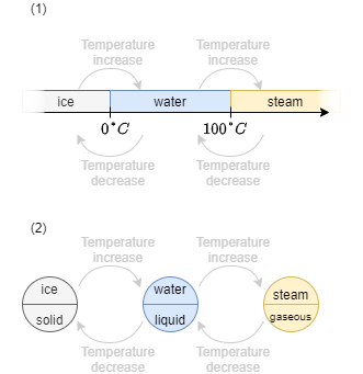
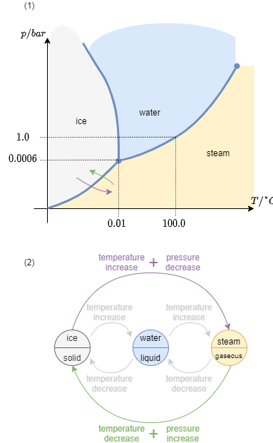
The diagrams of different states are well known from physics for example the state diagram (or better: phase diagram) of water, where its three states are: solid ice, liquid water and gaseous steam. The possible state transitions are due to temperature increase or decrease.
In figure 9 image (1) the states of water are shown on the temperature axis. When only the state transistions are relevant, the states are simplified to a circle, showing the state name and behaviour. The transitions are depict as arrows, where the needed condititon is written onto (See figure 9 image (2) ). This diagram is called state transition diagram.
For matter not only the dimension “temperature” is important, but also the “pressure”. The full phase diagram is shown in figure 10 image (1). By this, another variable is available and more transistions. These can be drawn into the state transition diagram (figure 10 image (2)).
6.3.2 Simple logic Example
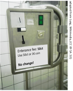
In German, often one has to pay for entering the toilet. An example of such a entrance control system is shown in figure 11. At this (artificial) example, one can pay either 50ct or 1€.
Once paid, the turnstile will release and one can enter. Once the turnstile was pushed the entrance is closed again.
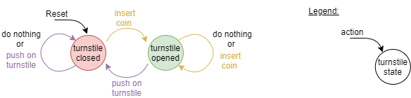
The figure 12 the state transition diagram is drawn.
- The two states are that (1) the turnstile is opened and one is able to go through and (2) the turnstile is closed and one cannot enter anymore.
- The transitions are given by the done actions: one can either insert a coin or push on the turnstile.
Important here are some additional considerations:
- For the state transition diagram one has to look for all possible transitions. So, also pushing a closed turnstile or inserting more coins have to taken into account.
- A state transition diagram is not complete without a legend and without an beginning/reset point. The reset point is given by an arrow with “reset” written onto it
Out of this state transition diagram one can create a table-like representation, see figure 13.
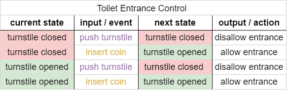
the inputs, outputs and states have to be encoded into binary, in order to investigate this table a bit more. How the binary value is connected to the outputs does not matter. We will choose the following coding:
- Encoding of the states: turnstile closed ≙ $Z=0$, turnstile opened ≙ $Z=1$,
- Encoding of the inputs: no coin inserted ≙ $Xc=0$, coin inserted ≙ $Xc=1$, turnstile not pushed ≙ $Xp=0$, turnstile pushed ≙ $Xp=1$,
- Encoding of the outputs: disallow entrance ≙ $Y=0$, allow entrance ≙ $Y=1$,
This table is shown in figure 14 and is called state transition table.
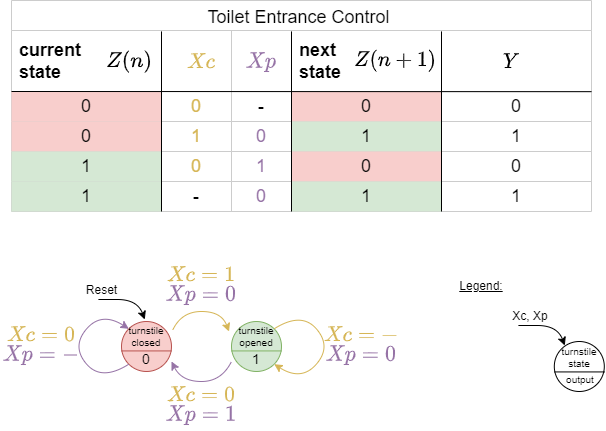
Interestingly, the logic circuit for this state transition table was already part of the course: it is the RS flip-flop! When looking deeper onto the table in figure 14 one can substitute $Xc$ with $S$ (as in Set) and $Xp$ with $R$ (as in Reset) to directly get the truthtable of the RS flip flop.
6.3.3 First Adaption for Up-Counter
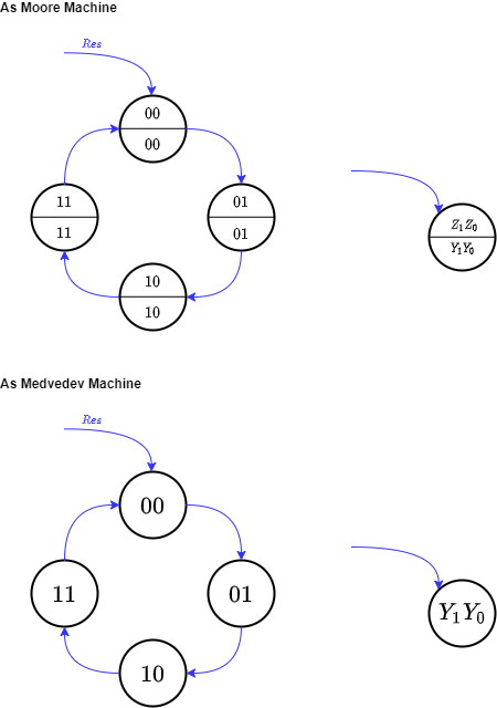
In the previous sub-chapter (6.2) we had a look onto different implementations of an up counter and on this chapter the way to represent a state machine via a state transition diagram. So one question is: how does these up counter look like in the state transition diagram?
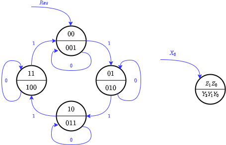
The Answer ist quite simple: there are 4 states, so 4 “circles” are needed. These states need to have circular connections in order to get the wanted increase from $%00=0$, to $%01=1$, to $%10=2$, to $%11=3$ and then back to $%00=0$. The first state shall be $%00=0$, so after the reset the state machine will get entered there. Finally, the output vector is similar to the state vector. With a deeper look onto is: This is therefore in particular a Medvedev machine!
In figure 15 both types of state machines are shown.
- In the Moore Machine the already seen “halving of the circle” is used to show the distinct state vector in the upper half and the output vector in the lower half.
- In the Medvedev Machine only one value is written in the circle, since here the state vector is also the output vector.
Exercise 6.3.3.1. State Transition Diagram in Digital.exe
The shown state transistion diagram can easily be created in the tool Digital:
- Click on the menu
Analysis»Finite State Machine - Here one either can add new states with a right click, or - more easier - go to the menu
Create»Create Counter»4 States - A (up) counter will get created
Tasks:
- Make the state machine get alive:
- Click to the menu
Create»State Transition Tablein order to see the state transition table - Here, click on the menu
Create»Cicruit - Now, the circuit can be started via the start button. The present state in the state transition diagram will also get highlighted.
The next step is to transform this into a up counter from $1...4$. For this simply the output has to be changed. This means the numbers in the “lower half of the circles” have to be adapted (see in <imfref pic16>).
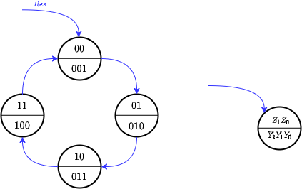
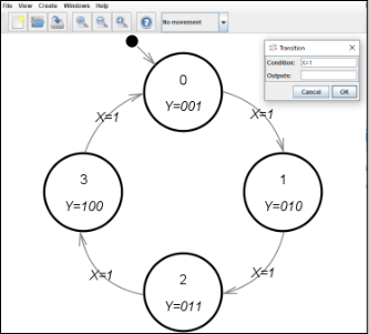
Exercise 6.3.3.2. State Transition Diagram II in Digital.exe
This exercise directly attached onto Exercise 6.3.3.2
The counter shall now be changed in such a way, that it counts $1 - 2 - 3 - 4$. For this: right click on each present states beginning with state 0 and add for Outputs $Y=001$ and upcounting (see image).
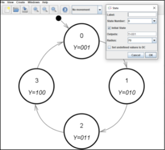
Tasks:
- Make this state machine again get alive
- Look at the circuit: Is it a Moore, Mealy or a Medvedev machine?
Looking on what we got, there is one part missing: the state machine does not have any input.. So the input vectors have to be added onto the transition (arrows). For an activateable counter, there only have to be one input $X$, which acts as an enable input.
Exercise 6.3.3.3. State Transition Diagram III in Digital.exe
This exercise directly attached onto Exercise 6.3.3.2
The last step is to add the transitions: right click on all transitions and add $X=1$ as a Condition.
Tasks:
- Make this state machine again get alive
Exercise 6.3.3.4. State Transition Diagram III in Digital.exe
This exercise directly attached onto Exercise 6.3.3.3
With the state machine in 6.3.3.3 it is also possible to create a state machine which can resemble a traffic light state machine. This shall transit from red, to red-yellow, to green, to yellow and then back to red.
Use the following addition to the resulting citcuit in order to get the light running:
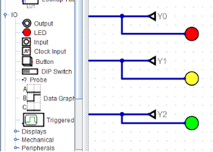
Tasks:
- Think about the right way to change the outputs in the state machine.
- Implement the needed correction and test the state machine.
Exercises
Exercise 6.1.1. State Transition Diagram I - fill the gaps
The following state transistion diagram shall be given:
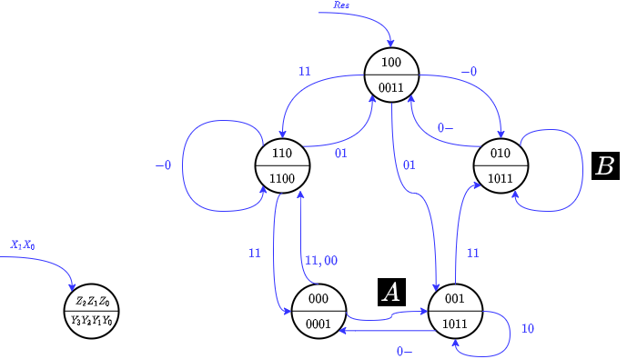
- There are two transitions marked with $A$ and $B$. What values does the inputs need to have in order show all transistions explicitely?
- How many flipflops are necessary for such a Moore Machine?
- Fill in the missing cells in the following state transition table:
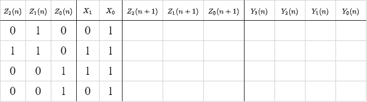
Exercise 6.1.2. State Transition Diagram II - Sequence
Design a state machine, which result in an output of the following (decimal) numbers: $4 - 5 - 2 - 1 - 6 - 7 - 0 - 3 - 4 - ...$
- The numbers shall repeat cyclic and without any other input than the clock $CLK$
- Draw the state transition diagram and the state transition table
- Use alternatively the structure of a 3bit up-counter
- Draw the structure of this moore machine with the up-counter as a blackbox, the input and output values and - if necessary - further blackboxes
- draw and fill in the additional table.
Exercise 6.1.3. State Transition Diagram III - Milling Machine
Design a state transistion diagram for a automatic milling machine as Moore machine, under the following conditions:
- The milling machine has 4 states: Initialisation $I$, Component Change $C$, Running $R$, Error $E$
- The milling machine starts at the state $I$.
- Once a limit switch $L$ is read as activated, the state $E$ shall be entered, independent which state the machine was in.
- Only in the state $E$ an alarm shall ring $A=1$.
- $E$ can only be exited with a reset.
- In order to change from Component Change $C$ to Running $R$, the user has to activate a Key $K=1$.
- Only when the machine is running $R$ and the Fixed Condition is reached $F=1$, the state Component Change $C$ shall be entered.
- Initialisation $I$ only changes into Component Change $C$, when no limit switch $L$ is activated and the Key is deactivated (input $K=0$) and the Fixed Condition is reached $F=1$.
Explicitely draw all possible transitions.
Exercise 6.1.4. State Transition Diagram IV - Find a sequence
Develop a sequential circuit, which creates the following output
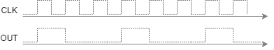
- Draw the state transition diagram of the moore machine of the synchronous sequential circuit.
- Create the digital ciruit.
Exercise 6.1.5. State Transition Diagram V - LED Fun
Develop a sequential circuit, which allows driving the following LED sequence
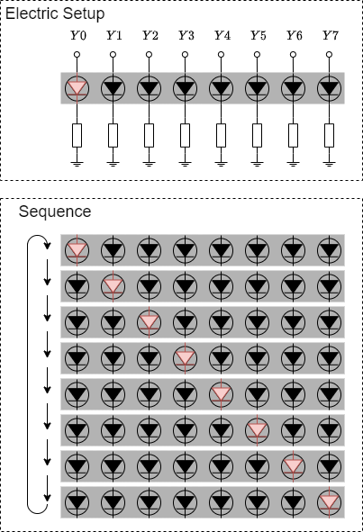
- Draw the state transition diagram of the moore machine of the synchronous sequential circuit.
- Create the digital ciruit.
Exercise 6.1.6. State Transition Diagram VI - Roll the dice
Develop a sequential circuit, which generate a clock driven up-counter from 1..6. The not reqired states shall lead after one clock cycle to the state of number 1 .
- Draw the state transition diagram of the moore machine of the synchronous sequential circuit.
- Create the digital ciruit.