Inhaltsverzeichnis

Block 05 — Resistive networks

Block 05 — Resistive networks

Learning objectives

After this 90-minute block, you can

reduce series/parallel resistor networks to an equivalent resistance $R_{\rm eq}$,
apply voltage divider (unloaded & loaded) and current divider rules,
recognize and analyze bridge circuits (Wheatstone; balance condition),
check results by units and by “sanity bounds” (e.g., $R_{\rm eq}$ in parallel is below the smallest branch).

90-minute plan

0–10 min — Recap KCL/KVL; sign conventions.
10–30 min — Series & parallel; quick numeric checks.
30–55 min — Voltage dividers (unloaded → loaded); potentiometer view; pitfalls.
55–70 min — Current divider; typical use.
70–85 min — Bridge circuits; balance; measurement idea.
85–90 min — Wrap-up quiz; assign exercises.

Core Content

Unloaded voltage divider

The series circuit of two resistors $R_1$ and $R_2$ shall be considered now.
This situation occurs in many practical applications e.g. in a potentiometer.

Abb. 1: potentiometer electrical_engineering_and_electronics_1:poti.svg

In Abbildung 2 this circuit is shown.

Abb. 2: unloaded voltage divider electrical_engineering_and_electronics_1:unbelasteterspannungsteiler.svg

Via Kirchhoff's voltage law, we get

$\boxed{ {{U_1}\over{U}} = {{R_1}\over{R_1 + R_2}} \rightarrow U_1 = k \cdot U}$

The ratio $k={{R_1}\over{R_1 + R_2}}$ also corresponds to the position on a potentiometer.

Exercise

Abb. 3: unloaded voltage divider

In the simulation in Abbildung 3 an unloaded voltage divider in the form of a potentiometer can be seen. The ideal voltage source provides $5~\rm V$. The potentiometer has a total resistance of $1~\rm k\Omega$. In the configuration shown, this is divided into $500 ~\Omega$ and $500 ~\Omega$.

What voltage $U_{\rm O}$ would you expect if the switch were closed? After thinking about your result, you can check it by closing the switch.
First, think about what would happen if you would change the distribution of the resistors by moving the wiper („intermediate terminal“).
You can check your assumption by using the slider at the bottom right of the simulation.
At which position do you get a $U_{\rm O} = 3.5~\rm V$?

The loaded Voltage Divider

If - in contrast to the abovementioned, unloaded voltage divider - a load $R_{\rm L}$ is connected to the output terminals (Abbildung 4), this load influences the output voltage.

Abb. 4: loaded voltage divider electrical_engineering_and_electronics_1:belasteterspannungsteiler.svg

A circuit analysis yields:

$ U_1 = \LARGE{{U} \over {1 + {{R_2}\over{R_L}} + {{R_2}\over{R_1}} }}$

or on a potentiometer with $k$ and the sum of resistors $R_{\rm s} = R_1 + R_2$:

$ U_1 = \LARGE{{k \cdot U} \over { 1 + k \cdot (1-k) \cdot{{R_{\rm s}}\over{R_{\rm L}}} }}$

Abbildung 5 shows the ratio of the output voltage $U_1$ to the input voltage $U$ (y-axis), in relation to the ratio $k={{R_1}\over{R_1 + R_2}}$. In principle, this is similar to Abbildung 2, but here it has another dimension: multiple graphs are plotted. These differ by the ratio ${{R_{\rm s}}\over{R_{\rm L}}}$.

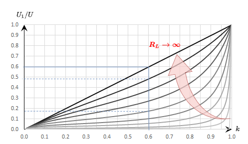
Abb. 5: Voltage curve of the loaded voltage divider electrical_engineering_and_electronics_1:spannungsverlaufbelasteterspannungsteiler.png

What does this diagram tell us? This shall be investigated by an example. First, assume an unloaded voltage divider with $R_2 = 4.0 ~\rm k\Omega$ and $R_1 = 6.0 ~\rm k\Omega$, and an input voltage of $10~\rm V$. Thus $k = 0.60$, $R_s = 10~\rm k\Omega$ and $U_1 = 6.0~\rm V$. Now this voltage divider is loaded with a load resistor. If this is at $R_{\rm L} = R_1 = 10 ~\rm k\Omega$, $k$ reduces to about $0.48$ and $U_1$ reduces to $4.8~\rm V$ - so the output voltage drops. For $R_{\rm L} = 4.0~\rm k\Omega$, $k$ becomes even smaller to $k=0.375$ and $U_1 = 3.75~\rm V$. If the load $R_{\rm L}$ is only one-tenth of the resistor $R_{\rm s}=R_1 + R_2$, the result is $k = 0.18$ and $U_1 = 1.8~\rm V$. The output voltage of the unloaded voltage divider ($6.0~\rm V$) thus became less than one-third.

What is the practical use of the (loaded) voltage divider?
Here are some examples:

Voltage dividers are in use for controlling the output of power supply ICs (see Voltage Dividers in Power Supplies). In order not to create a loaded voltage divider, a range for the resistance is given here.
Another „invisible“ voltage divider is for example in the electrical system of a car. As we will learn in the next chapters, voltage supplies have internal resistance (and therefore batteries, too). The other consumer in the car also represents a resistance. By this, the electrical system states an unloaded voltage divider. Given another, additional low-resistance load (e.g. the spark or the starter motor of the starter system) one can understand that there will be a voltage drop when starting the car.

Bridge networks (Wheatstone)

A four-resistor bridge can be seen as two voltage dividers in parallel. The detector (bridge branch) sees the difference of the two divider node voltages. The balance condition (zero detector current) is \begin{align*} \boxed{ \frac{R_1}{R_2}=\frac{R_3}{R_4} \;\; \Leftrightarrow \;\; R_1R_4=R_2R_3 }. \end{align*} Use this to check sensor bridges (strain gauges etc.) or to compute unknown $R$. (Derivation via equal divider ratios.)

If the bridge is nearly balanced, the midpoint voltages differ only slightly → good for small-signal sensing.
In practice you’ll later buffer such nodes with high-$R_{\rm in}$ stages (see op-amps in Block21).

Strategy for network reduction

Reshape (without changing node connections), then collapse clear series or parallel groups.
If blocked by a three-terminal cluster, apply Δ–Y (or Y–Δ), then collapse again.
Repeat until a simple ladder remains; finish with KCL/KVL if needed.

In this subchapter, a methodology is discussed, which should help to reshape circuits. The following concept works at tasks, where the total resistance, total current, or total voltage has to be calculated for a resistor network.

An example of such a circuit is given in Abbildung 6. Here $I_0$ is wanted. This current can be found by the (given) voltage $U_0$ and the total resistance between the terminals $\rm a$ and $\rm b$. So we are looking for $R_{\rm ab}$.

Abb. 6: example of a circuit electrical_engineering_and_electronics_1:beispielstromkreis2.svg

As already described in the previous subchapters, partial circuits can also be converted into equivalent resistors step by step. It is important to note that these partial circuits for conversion into equivalent resistors may only ever have two connections (= two nodes to the „outside world“).

Abb. 7: Step-by-step solution of the example electrical_engineering_and_electronics_1:beispielstromkreis2loesung.svg

Abbildung 7 shows the step-by-step conversion of the equivalent resistors in this example.
As a result of the equivalent resistance one gets:

\begin{align*} R_{\rm eq} = R_{12345} &= R_{12}||R_{345} = R_{12}||(R_3+R_{45}) = (R_1||R_2)||(R_3+R_4||R_5) \\ &= {{ {{R_1 \cdot R_2}\over{R_1 + R_2}} \cdot (R_3 + {{R_4 \cdot R_5}\over{R_4 + R_5}}) }\over{ {{R_1 \cdot R_2}\over{R_1 + R_2}} +R_3 + {{R_4 \cdot R_5}\over{R_4 + R_5}} }} \quad \quad \quad \quad \quad \quad \bigg\rvert \cdot{{(R_1 + R_2) \cdot (R_4 + R_5)}\over{(R_1 + R_2) \cdot (R_4 + R_5)}} \\ &= {{ R_1 \cdot R_2 \cdot (R_3 + {{R_4 \cdot R_5}\over{R_4 + R_5}}) \cdot (R_4 + R_5) } \over { R_1 \cdot R_2\cdot(R_4 + R_5) +R_3 + R_4 \cdot R_5 \cdot (R_1 + R_2)}} \\ &= {{ R_1 \cdot R_2 \cdot (R_3 \cdot (R_4 + R_5) + R_4 \cdot R_5) } \over { R_1 \cdot R_2\cdot(R_4 + R_5) +R_3 + R_4 \cdot R_5 \cdot (R_1 + R_2)}} \\ \end{align*}

Exercises

Exercise 2.4.3 Three Resistors

Three equal resistors of $20~k\Omega$ each are given.
Which values are realizable by the arbitrary interconnection of one to three resistors?
Solution

The resistors can be connected in series: \begin{equation*} R_{\rm series} = 3\cdot R = 3\cdot20~k\Omega \end{equation*} The resistors can also be connected in parallel: \begin{equation*} R_{\rm parallel} = \frac{R}{3} = \frac{20~k\Omega}{3} \end{equation*} On the other hand, they can also be connected in a way that two of them are in parallel and those are in series to the third one: \begin{equation*} R_{\rm res} = R + \frac{R\cdot R}{R+R} = \frac{3}{2}R = \frac{3}{2} \cdot 20~k\Omega \end{equation*}

Final values

\begin{equation*} R_{series} = 60~k\Omega\qquad R_{\rm parallel} = 6.7~k\Omega\qquad R_{\rm res} = 30~k\Omega \end{equation*}

Exercise 2.5.2 loaded voltage divider I

Determine from the circuit in Abbildung 4 the equation $ U_1 = {{k \cdot U} \over { 1 + k \cdot (1-k) \cdot{{R_{\rm s}}\over{R_{\rm L}}}}}$ where $k={{R_1}\over{R_1 + R_2}}$ and $R_{\rm s} = R_1 + R_2$.
Solution

According to the voltage division rule, the loaded voltage is \begin{align*} U_1 &=\frac{\frac{R_1 R_L}{R_1+R_L}}{R_2+\frac{R_1 R_L}{R_1+R_L}}U \\ &=\frac{R_1 R_{\rm L}}{R_2 (R_1 + R_{\rm L}) + R_1 R_{\rm L}} U \\ &=\frac{R_1 R_{\rm L}}{R_1 R_2 + R_2 R_{\rm L} + R_1 R_{\rm L}} U \\ &=\frac{R_1 R_{\rm L}}{R_1 R_2 + (R_1+R_2) R_{\rm L}} U \end{align*} The divided resistor $R_1$ and $R_2$ are put together to form $R_{\rm s}=R_1 + R_2$. \begin{equation*} U_1=\frac{R_1 R_{\rm L}}{R_1 R_2 + R_{\rm s} R_{\rm L}} U \end{equation*} With the equations given there is also $R_1=k(R_1+R_2)=k R_{\rm s}$ and $R_2 = R_{\rm s} - R_1 = R_{\rm s} - k R_{\rm s} = (1-k) R_{\rm s}$. \begin{equation*} U_1=\frac{k R_{\rm s} R_{\rm L}}{k R_{\rm s} (1-k) R_{\rm s} + R_{\rm s} R_{\rm L}}U \end{equation*} Dividing the numerator and denominator by $R_{\rm s} R_{\rm L}$ yields to \begin{equation*} U_1=\frac{k}{k(1-k)\frac{R_{\rm s}}{R_{\rm L}}+1}U \end{equation*}

Exercise 2.5.3 loaded voltage divider II

In the simulation in Abbildung 8 a loaded voltage divider in the form of a potentiometer can be seen. The ideal voltage source provides $5.00~\rm V$. The potentiometer has a total resistance of $1.00~k\Omega$. In the configuration shown, this is divided into $500 ~\Omega$ and $500 ~\Omega$. The load resistance has $R_{\rm L} = 1.00 ~\rm k\Omega$.

What voltage U_O would you expect if the switch were closed? This is where you need to do some math! After you calculated your result, you can check it by closing the switch.
At which position of the wiper do you get $3.50~\rm V$ as an output? Determine the result first by means of a calculation.
Then check it by moving the slider at the bottom right of the simulation.

Abb. 8: loaded voltage divider

Exercise 2.5.4 Application of the loaded voltage divider - motor

Abb. 9: Sketch of the setup
electrical_engineering_and_electronics_1:motoramspannungsteiler.svg

You wanted to test a micromotor for a small robot. Using the maximum current and the internal resistance ($R_{\rm M} = 5~\Omega$) you calculate that this can be operated with a maximum of $U_{\rm M, max}=4~\rm V$. A colleague said that you can get $4~\rm V$ using the setup in Abbildung 9 from a $9~\rm V$ block battery.

First, calculate the maximum current $I_{\rm M,max}$ of the motor.
Draw the corresponding electrical circuit with the motor connected as an ohmic resistor.
At the maximum current, the motor should be able to deliver a torque of $M_{\rm max}=M(I_{\rm M, max})= 100~\rm mNm$. What torque would the motor deliver if you implement the setup like this? (Assumption: The torque of the motor increases proportionally to the motor current).
What might a setup with a potentiometer look like that would actually allow you to set a voltage between $0.5~\rm V$ to $4~\rm V$ on the motor? What resistance value should the potentiometer have?
Build and test your circuit in the simulation below. For an introduction to online simulation, see: online_circuit_simulator.
You will essentially need the following tips for this setup:
1. Routing connections can be activated via the menu: Draw » add wire. Afterward, you have to click on the start point and then drag it to the end mode.
2. Note that connections can only ever be connected at nodes. A red-marked node (e.g. at the $5 ~\Omega$ resistor) indicates that it is not connected. This could be moved one grid step to the left, as there is a node point there.
3. Pressing the <ESC> key will disable the insertion of components.
4. With a right click on a component it can be copied or values like the resistor can be changed via Edit….

Abb. 10: Simulation for motor setup

Exercise 2.5.5 Examples of the calculation of loaded voltage dividers

Exercise on the voltage divider

Exercise 2.5.6 Example of a loaded voltage divider: Explanation without calculation (German)

Exercise 2.7.1 Circuit Simplification Exercise I (in German)

Exercise 2.7.2 Circuit Simplification Exercise II + III (in German)

Exercise 2.7.3 Circuit Simplification Exercise IV (in German)

Exercise 2.7.4 Circuit Simplification Exercise V (in German)

Exercise 2.7.5 Circuit Simplification Exercise VI (in German)

Exercise 2.7.7 Simplifying Circuits (exam task, about 8% of a 60-minute exam, WS2020)

Given is the adjoining circuit with
$R_1=10 ~\Omega$
$R_2=20 ~\Omega$
$R_3=5 ~\Omega$
and the switch $S$.

1. Determine the total resistance $R_{\rm eq}$ between A and B by summing the resistances with the switch $S$ open.

Tips for solving

How can the circuit be better represented or pulled apart?
The switch should be replaced by an open wire in this case.

Solution

First of all, it is a good idea to reshape the circuit so that the actual structure becomes visible.
For this purpose, the individual branches can be highlighted in color and interpreted as a „conductive rubber band“.
This results in:

Thus $R_3$ and $R_3$ can be combined to $R_{33} = 2 \cdot R_3 = R_1$, yielding a left and a right voltage divider.
Now it is visible that in the left and right voltage divider, the same potential is at the respective branch, or at the node K1 (green) and K2 (pink).

Thus, the total resistance can be calculated as $R_{\rm eq} = (2 \cdot R_1)||(2 \cdot R_1)$.
However, by symmetry, nodes K1 and K2 can also be short-circuited. Thus, $R_{\rm eq} = 2 \cdot \left( R_1||R_1 \right)$ also holds.

Final result

\begin{align*} R_{\rm eq} &= 2 \cdot \left( 10 ~\Omega || 10 ~\Omega \right) = 10 ~\Omega \end{align*}

2. What is the total resistance when switch $S$ is closed?

Final result

Due to symmetry, the potentials at K1 and K2 are equal. Thus, no current flows across resistor $R_2$ even when the switch is closed.
So the resistance remains the same.

Exercise 2.7.8: Simplifying Circuits II (written exam task, approx 8% of a 60-minute written exam, WS2020)

Given is the adjoining circuit with
$R_1=5 ~\Omega$
$R_2=10 ~\Omega$
$R_3=20 ~\Omega$

1. Determine the equivalent resistance $R_{\rm eq}$ between A and B by summing the resistances.

Tips for solving

How can the circuit be better represented or pulled apart?
Switches (when used) should be replaced by an open or closed circuit.
Does this result in equal potentials at different nodes that can be cleverly used?

Solution

Here it helps to consider the potential of the nodes K1, K2, and K3. For K2, the resistances $R_2 || R_3 || R_2$ must be combined at the top and bottom. Thus, the same resistance values at the top and bottom result. Also at the nodes K1 and K2 the same resistance values at the top and at the bottom result. With the same ratios of the resistances at K1, K2, and K3 respectively, it can be concluded that no current flows across the resistors $R_3$ between K1 and K2 or K2 and K3. Thus, these do not contribute to the total resistance. In such a case, a short circuit or an open line can be freely chosen between the relevant nodes for the calculation. In the following, an open line is chosen. Additionally, the parallel strings can be reordered.

Abb. 11: Simulation

This results in:

\begin{align*} R_{\rm eq} &= \left( \left( 2 \cdot R_2 \right) || \left( 2 \cdot R_2 \right) \right) && || \; \left( \left( 2 \cdot R_3 \right) || \left( 2 \cdot R_3 \right) || \left( 2 \cdot R_3 \right) \right) \\ R_{\rm eq} &= R_2 && || \;\left( R_3 || \left( 2 \cdot R_3 \right) \right) \\ R_{\rm eq} &= R_2 && || \;\frac{R_3 \cdot 2 R_3}{R_3 + 2 R_3} \\ R_{\rm eq} &= R_2 && || \;\frac{2}{3}\cdot R_3 \\ R_{\rm eq} &= \frac{R_2 \cdot \frac{2}{3}\cdot R_3}{R_2 + \frac{2}{3}\cdot R_3} \\ R_{\rm eq} &= \frac{R_2 \cdot R_3}{\frac{3}{2}\cdot R_2 + R_3} \\ \\ \end{align*}

Final result

\begin{align*} R_{\rm eq} &= \frac{10 ~\Omega \cdot 20 ~\Omega}{\frac{3}{2}\cdot 10 ~\Omega + 20 ~\Omega} = 5.7143 ~\Omega \rightarrow 5.7 ~\Omega \end{align*}

2. Now let the voltage from A to B be: $U_{AB}=U_0= 20 ~\rm V$. What is the current $I$?

Solution

The partial current $I$ is obtained directly from the voltage $U_0$: \begin{align*} I &=\frac{U_0}{2 \cdot R_3} \end{align*}

Final result

\begin{align*} I =\frac{20~V}{2 \cdot 20 ~\Omega} = 0.5 ~\rm A \end{align*}

Exercise 2.7.9 - Variation: Simplifying Circuits II (written exam task, approx 8% of a 60-minute written exam, WS2020)

Given is the adjoining circuit with
$R_1=10 ~\Omega$
$R_2=20 ~\Omega$
$R_3=5 ~\Omega$

1. Determine the equivalent resistance $R_{\rm eq}$ between A and B by summing the resistances.

Final result

\begin{align*} R_{ges} &= \frac{20 ~\Omega \cdot 5 ~\Omega}{\frac{3}{2}\cdot 20 ~\Omega + 5 ~\Omega} = 2.858 ~\Omega \rightarrow 2.9 ~\Omega \end{align*}

2. Now let the voltage from A to B be: $U_{\rm AB}=U_0= 10 ~\rm V$. What is the current $I$?

Final result

\begin{align*} I =\frac{10~\rm V}{2 \cdot 5 ~\Omega} = 1 ~\rm A \end{align*}

Exercise 2.7.10 - Variation: Simplifying Circuits III (written exam task, approx 8% of a 60-minute written exam, WS2020)

Given is the adjoining circuit with
$R_1=5 ~\Omega$
$R_2=20 ~\Omega$
$R_3=10 ~\Omega$

1. Determine the equivalent resistance $R_{\rm eq}$ between A and B by summing the resistances.

2. Now let the voltage from A to B be: $U_{\rm AB}=U_0= 30 ~\rm V$. What is the current $I$?

Embedded resources

Why are voltage dividers important? (a cutout from 0:00 to 10:56 from a full video of EEVblog, starting from 17:00 there is also a nice example for troubles with voltage dividers..)

Summary (take-away)

Series: $R$ adds; Parallel: $G$ adds.
Voltage divider: $U_1= \dfrac{R_1}{R_1+R_2}U$ (unloaded); with load, $U_1$ decreases per $\displaystyle U_1=\frac{U}{1+\frac{R_2}{R_{\rm L}}+\frac{R_2}{R_1}}$.
Current divider: branch currents split in proportion to conductances.
Bridge: balance when products of opposite arms are equal.
Δ–Y / Y–Δ: unlocks reductions when pure series/parallel isn’t available.

All formulas consistent with the colleague’s slides (ee1spo4.pdf ch.2).

Preparation for next block

Skim real sources & two-terminal networks (internal resistance, Thevenin/Norton). Bring questions about loaded dividers and efficiency vs. power transfer (ties into utilization/impedance matching).