In your company „HHN Mechatronics & Robotics“ you have built a single-ended rectifier to rectify a sinusoidal measuring signal of ($f=200~\rm kHz$, amplitude $\hat{U} = 5.0~\rm V$, output resistance of the sensor $R_{\rm q} = 10~\rm k\Omega$). For this purpose, you built a simple circuit with the „Si rectifier diode“ $D=\rm 1N5400$ and a smoothing capacitor with $C=10~\rm pF$. As a measuring instrument, you used an oscilloscope (Rigol DS1000E). The circuit is drawn in the adjacent sketch.

Your colleague has already pointed out to you that at high frequencies some diodes get a problem with rectification. You also noticed this when measuring the setup and looking at the oscilloscope…

Write down the expected signal curve before the respective simulation. Note that you must consider a steady-state system in the simulation!

1. Find in the Instruction of the oscilloscope the values of the input impedance, which are needed in the circuit for the input resistance $R_\rm E$ and the input capacitance $C_\rm E$.
   Replicate the circuit in using the information from TINA TI above (Circuit 1). Take into account the input impedance of the oscilloscope, as shown in the sketch.
   Simulate circuit 1 with the specified signal. Briefly describe the expected and measured signal waveforms.
2. Try tuning the capacitance of capacitor $C$ to get the expected rectified value. What do you find?
3. Since something seems to be funny, you want to debug the circuit, that is, determine the error. To do this, you could use the generic approach to debugging (in German). Or you break down the unclear system to a minimum. Specifically, you build a modified circuit (Circuit 2):
   1. the sensor is replaced by a function generator (same frequency and amplitude, but $R_{\rm q} = 50 ~\Omega$),
   2. the smoothing capacitor $C$ is replaced by an open lead (so it is no longer present)
4. Simulate circuit 2 with the signal given so far. Briefly describe the expected and measured signal characteristics.
5. Now take another step back and try to get a little more current flowing across the diode. In circuit 2, the current was limited by $R_\rm E$ and thus the diode was not yet operating above $U_\rm S=0.7~\rm V$. The idea now in Circuit 3 is to also switch the input resistor to $R_\rm E = 50 ~\Omega$ (this is possible on some oscilloscopes). The rest of circuit 3 is the same as circuit 2. Simulate circuit 3 with the signal given so far.
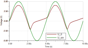
6. Now you seem to be getting closer to the problem. You vary input resistance to $R_\rm E = 500 ~\Omega$ (Circuit 4)
   Simulate circuit 4 with the given signal. Briefly describe the expected and measured signal waveforms.
7. Your colleague tips you that the progression (see diagram on the right) is typical of
   1. A reverse recovery time $t_{\rm rr}$ that is too large. This is reproduced in Tina via the transit time $\rm TT$.
   2. an excessive junction capacity (junction capacity $C_\rm j$ or diode capacity $C_\rm D$).
8. These values can be changed in Tina TI by the following procedure: Double-click on the diode » click on … at Type » search for the mentioned values.
   You now want to analyze how the reverse bias and the junction capacitance affect the voltage curve (for circuit 4).
   Simulate and describe the voltage curve if
   1. on the one hand, the reverse bias is reset to $0~\rm s$ or
   2. on the other hand, the junction capacitance is reset to $0~\rm F$.
      describe the voltage waveform.
9. Instead of diode $D=\rm 1N5400$, choose diode $D=\rm 1N4148$ and simulate again circuit 3 and circuit 1.
   Now how does the voltage waveform behave and why?