This is an old revision of the document!
7. Networks at variable frequency
Further content can be found at elektroniktutor
Introduction
At the previous chapters it was explained how the “influence of a sinusoidal current flow” of capacitor and inductors look like. To describe this, the impedance was introduced. This can be understood as a complex resistance for sinusoidal excitation.
It applies to the capacitor:
\begin{align*} \underline{U}_C = \frac{1}{j\omega \cdot C} \cdot \underline{I}_C \quad \rightarrow \quad \underline{Z}_C = \frac{1}{j\omega \cdot C} \end{align*}
and for the inductance
\begin{align*} \underline{U}_L = j\omega \cdot L \cdot \underline{I}_L \quad \rightarrow \quad \underline{Z}_L = j\omega \cdot L \end{align*}
Complex impedances can be dealt with in much the same way as ohmic resistances in Electrical Engineering 1 (see: simple_dc_circuits, linear_sources_and_bipoles, analysis_of_dc_networks). In these transformations, the fraction $ j\omega \cdot$ is preserved. Circuits with impedances such as inductors and capacitors will show a frequency dependence accordingly.
7.1 Frequency-dependent voltage divider
Targets
After this lesson, you should:
- know that …
- know that … is formed.
- be able to … can …
From two-pole to four-pole
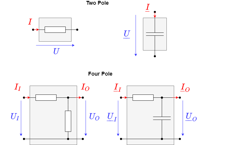
Until now, components such as resistors, capacitors and inductors have been understood as two-terminal. This is also obvious, since there are only two connections. In the following however circuits are considered, which behave similar to a voltage divider: On one side a voltage $U_E$ is applied, on the other side $U_A$ is formed with it. This results in 4 terminals. The circuit can and will be considered as a four-terminal circuit in the following. But the input and output values will be complex.
For quadripoles, the relation of “what goes out” (e.g. $\underline{U}_O$ or $\underline{U}_2$) to “what goes in” (e.g. voltage $\underline{U}_I$ or $\underline{U}_1$) is important. Thus, the output and input variables ($\underline{U}_O$) and ($\underline{U}_I$) give the quotient:
\begin{align*} \underline{A} & = \frac {\underline{U}_O}{\underline{U}_I} \\ & \text{with} \; \underline{U}_O = U_O \cdot e^{j \varphi_{uO}} \\ & \text{and} \; \underline{U}_I = U_I \cdot e^{j \varphi_{uI}} \\ \\ \underline{A}& = \frac {\underline{U}_O}{\underline{U}_I} = \frac {U_O \cdot e^{j \varphi_{uO}}}{U_I\cdot e^{j \varphi_{uI}}} \\ & = \frac {U_O}{U_I}\cdot \cdot e^{j (\varphi_{uO}-\varphi_{uI})} \\ \end{align*} \begin{align*} \boxed{\underline{A} = \dfrac {\underline{U}_O}{\underline{U}_I} = \frac {U_O}{U_I}\cdot e^{j \Delta\varphi_{u}}} \end{align*}
Note:
- The complex-valued quotient ${\underline{U}_O}/{\underline{U}_I}$ is called the transfer function.
- The frequency-dependent magnitude of the quotient $A(\omega)={U_O}/{U_I}$ is called amplitude response and the angular difference $\Delta\varphi_{u}(\omega)$ is called phase response.
The frequency behaviour of the amplitude response and the frequency response is not only important in electrical engineering and electronics, but will also play a central role in control engineering.
RL series connection
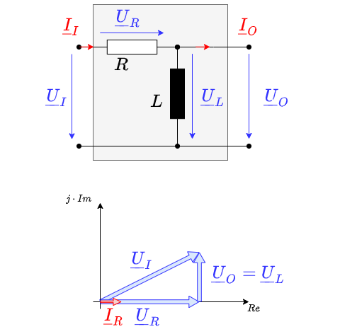
First, a series connection of a resistor $R$ and an inductor $L$ shall be considered (see figure 2). This structure is also called RL-element.
Here, $\underline{U}_I= \underline{X_I} \cdot \underline{I}_I$ with $\underline{X}_I = R + j\omega \cdot L$ and corresponding for $\underline{U}_O$: \begin{align*} \underline{A} = \dfrac {\underline{U}_O}{\underline{U}_I} = \frac {\omega L}{\sqrt{R^2 + (\omega L)^2}}\cdot e^{j\left(\frac{\pi}{2} - arctan \frac{\omega L}{R} \right)} \end{align*}
This results in the following for
- the amplitude response: $A = \frac {\omega L}{\sqrt{R^2 + (\omega L)^2}}$ and
- the phase response: $\Delta\varphi_{u} = \frac{\pi}{2} - arctan \frac{\omega L}{R}$
The main focus should first be on the amplitude response. Its frequency response can be derived from the equation in various ways.
- Limit value consideration of the RL arrangement (in the equation and in the system)
- Plotting amplitude and frequency response
- Determination of prominent frequencies
These three points are now to be gone through.
Limit value consideration of the RL arrangement
For the limit consideration we look at what, happens when the frequency $\omega$ runs to the definition range limits, i.e. $\omega \rightarrow 0$ and $\omega \rightarrow \infty$:
- For $\omega \rightarrow 0$, $A = \frac {\omega L}{\sqrt{R^2 + (\omega L)^2}} \rightarrow 0$ as the numerator approaches zero and the denominator remains greater than zero.
- For $\omega \rightarrow \infty$, $A \rightarrow1$, because in the root in the denominator $(\omega L)^2$ becomes larger and larger in the ratio $R^2$ to . So the root tends to $\omega L$ and thus to the numerator.
It can thus be seen that:
- at small frequencies there is no voltage $U_2$ at the output.
- at high frequencies $A = \frac {U_O}{U_I} = \rightarrow 1$, so the voltage at the output is equal to the voltage at the input.
The RL element shown here therefore only allows large frequencies to pass (= pass through) and small ones are filtered out. The circuit corresponds to a high pass.
This can also be derived from understanding the components: At small frequencies, the current in the coil and thus the magnetic field changes only slowly. So only a negligibly small reverse voltage is induced. The coil acts like a short circuit at low frequencies. At higher frequencies, the current generated by $U_I$ through the coil changes faster, the induced voltage $U_i = - dI / dt$ becomes large. As a result, the coil inhibits the current flow and a voltage drops across the coil. If the frequency becomes very high, only a negligible current flows through the coil - and hence through the resistor. The voltage drop at $R$ thus approaches zero and the output voltage $U_O$ tends towards $U_I$.
For further consideration, the equation of the transfer function $\underline{A} = \dfrac {\underline{U}_O}{\underline{U}_I}$ is to be rewritten so that it becomes independent of component values. This allows for a generalized representation. This representation is called normalization:
\begin{align*} \underline{A} = \dfrac {\underline{U}_O}{\underline{U}_I} = \frac {\omega L}{\sqrt{R^2 + (\omega L)^2}}\cdot e^{j\left(\frac{\pi}{2} - arctan \frac{\omega L}{R} \right)} \quad \xrightarrow{\text{normalization}} \quad \quad \underline{A}_{norm} = \frac {\omega L / R}{\sqrt{1 + (\omega L / R)^2}}\cdot e^{j\left(\frac{\pi}{2} - arctan \frac{\omega L}{R} \right)} = \frac {x}{\sqrt{1 + x^2}} \cdot e^{j\left(\frac{\pi}{2} - arctan x \right)} \end{align*}
This equation behaves quite the same as the one considered so far.
<WRAP>
\\  === Plotting amplitude and frequency response ===
</WRAP>
The transfer function can also be decomposed into amplitude response and frequency response. This can be done by
- the amplitude response double logarithmic and
- the phase response single logarithmic
logarithmically. figure 4 shows the two plots. On the x-axis, $x = \omega L / R$ has been plotted as the normalization variable. This represents a weighted frequency.
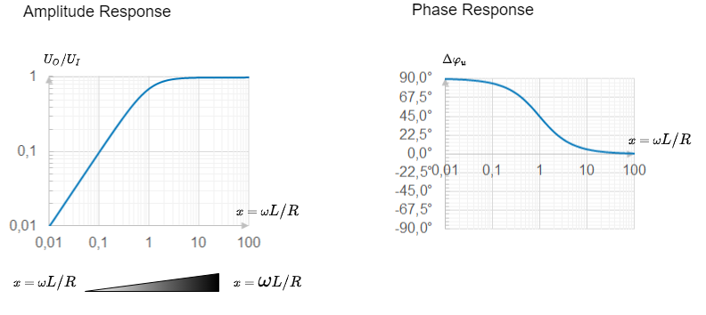
Here, too, the behavior determined in the limit value observation can be seen: at small frequencies $\omega$ (corresponds to small $x$), the amplitude response tends toward zero. At high frequencies, the ratio $U_O / U_I = 1 $ is established.
Interesting in the phase response is the point $x = 1$.
- Further to the left of this point (i.e. at smaller frequencies) a tenfold increase of the frequency $\omega$ produces a tenfold increase of $U_O / U_I$.
- Further to the right of this point (i.e. at higher frequencies) $U_O / U_I = 1$ remains.
So this point marks a limit. Far to the left, the ohmic resistance is significantly greater the amount of impedance of the coil: $R >> \omega L$. far to the right is just the opposite.
The point $x=1$ just marks the cutoff frequency. It holds
\begin{align*} \underline{A}_{norm} = \frac{x}{\sqrt{1 + x^2}}\cdot e^{j\left(\frac{\pi}{2} - arctan x \right)}= \frac {U_O}{U_I} \cdot e^{j\varphi}\quad \quad \left{ \begin{array} x \ll 1 & \widehat{=} \omega L \ll R &: \quad\quad \frac{U_O}{U_I}=x &, \varphi = \frac{\pi}{2} & \widehat{=} 90° x \gg 1 & \widehat{=} \omega L \gg R &: \quad\quad \frac{U_O}{U_I}=1 &, \varphi = 0 & \widehat{=} 0° x = 1 & \widehat{=} \omega L = R &: \quad\quad \frac{U_O}{U_I}=\frac{1}{\sqrt{2}} &, \varphi = \frac{\pi}{4} &, \widehat{=} 45{°}\end{array} \right.\end{align*}
Reminder:
- The cutoff frequency for high-pass and low-pass filters is the frequency at which the ohmic resistance just equals the value of the impedance.
- The cutoff frequency separates a range in which the filter allows signals through from one in which they are suppressed (=blocked).
- At the cutoff frequency, the phase $\varphi = 45°$ and the amplitude $A = \frac{1}{\sqrt{2}}$.
These statements apply to single-stage passive filters, i.e. one RL or one RC element. Multistage filters are considered in circuit engineering.
The cut-off frequency in this case is given by:
\begin{align*} R &= \omega L \omega_{Gr} &= \frac{R}{L} 2 \pi f_{Gr} &= \frac{R}{L} \quad \rightarrow \quad \boxed{f_{Gr} = \frac{R}{2 \pi \cdot L}} \end{align*}
SYNC, CORRECTED BY ELDERMAN
low pass
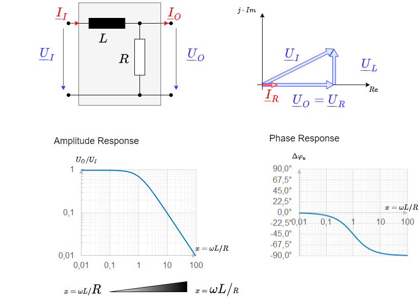
So far, only one variant of the RL element has been considered, namely the one where the output voltage $\underline{U}_A$ is tapped at the inductance. Here we will briefly discuss what happens when the two components are swapped.
In this case, the normalized transfer function is given by:
\begin{align*} \underline{A}_{norm} = \frac {1}{\sqrt{1 + (\omega L / R)^2}}\cdot e^{-j arctan \frac{\omega L}{R} } \end{align*}
The cutoff frequency is again given by $f_{Gr} = \frac{R}{2 \pi \cdot L}$.
RC Series
RC high pass
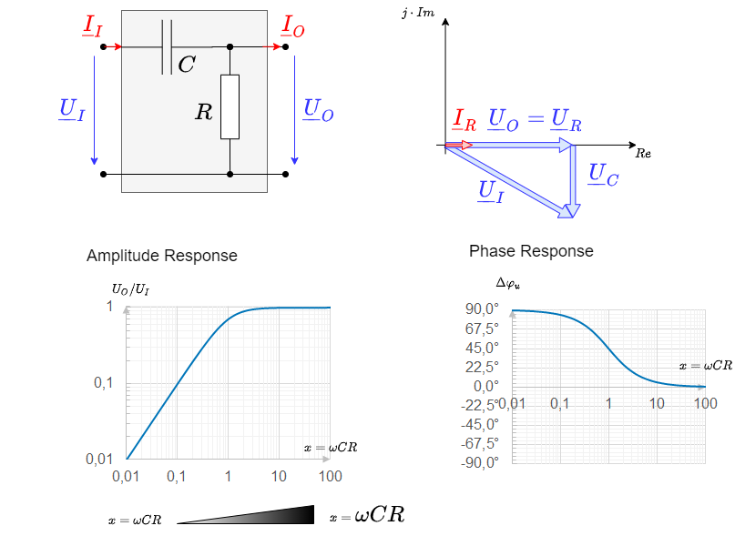
Now a voltage divider is to be constructed by a resistor $R$ and a capacity $C$. Quite similar to the previous chapters, the transfer function can also be determined here.
Here results as normalized transfer function:
\begin{align*} \underline{A}_{norm} = \frac {\omega RC}{\sqrt{1 + (\omega RC)^2}}\cdot e^{\frac{\pi}{2}-j arctan \omega RC } \end{align*}
In this case, the normalization variable $x = \omega RC$. Again, the cutoff frequency is determined by equating $R$ and the magnitude of the impedance of the capacitance:
\begin{align*} R &= \frac{1}{\omega_{Gr} C} \omega_{Gr} &= \frac{1}{RC} 2 \pi f_{Gr} &= \frac{1}{RC} \quad \rightarrow \quad \boxed{f_{Gr} =\frac{1}{2 \pi\cdot RC} } \end{align*}}
rc low pass
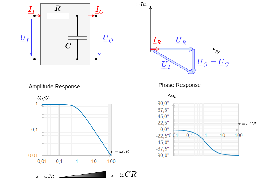
Again, the voltage at the impedance is to be used as the output voltage. This results in a low-pass filter.
Here results as normalized transfer function:
\begin{align*} \underline{A}_{norm} = \frac {1}{\sqrt{1 + (\omega RC)^2}}\cdot e^{-j arctan \omega RC } \end{align*}
Also, the cutoff frequency is given by $f_{Gr} =\frac{1}{2 \pi\cdot RC}$
7.2 Resonance phenomena
RLC - Series Resonant Circuit
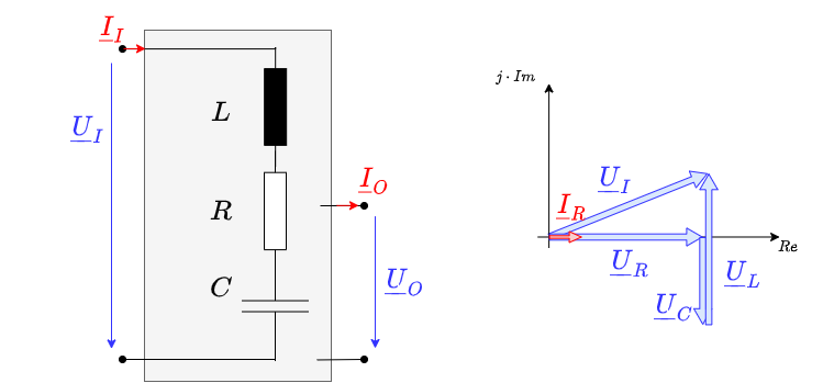
If a resistor $R$, a capacitor $C$ and an inductance $L$ are connected in series, the result is a series resonant circuit. In this case the output voltage is not clearly defined. It must be considered in the following how the voltages behave across the individual components. The total voltage (= input voltage $U_E$) results to:
\begin{align*} \underline{U} = \underline{U}_R + \underline{U}_L + \underline{U}_C \end{align*}
Since the current in the circuit must be constant, the total impedance can be determined here in a simple way:
\begin{align*} \underline{U} &= R \cdot \underline{I} + j \omega L \cdot \underline{I} + \frac {1}{j\omega C } \cdot \underline{I} \underline{U} &= \left( R + j \omega L - j \cdot \frac {1}{\omega C } \right) \cdot \underline{I} \underline{Z}_{ges} &= R + j \omega L - j \cdot \frac {1}{\omega C } \end{align*}
As the magnitude of the (input) voltage $U$ or the (input or total) impedance $Z$ and the phase result to:
\begin{align*} U &= \sqrt{U_R^2 + (U_Z)^2} = \sqrt{U_R^2 + (U_L - U_C)^2} \end{align*}
\begin{align*} Z &= \sqrt{R^2 + (Z)^2} = \sqrt{R^2 + (\omega L - \frac{1}{\omega C})^2} \end{align*}
\begin{align*} \varphi_u = \varphi_Z &= arctan \frac{\omega L - \frac{1}{\omega C}}{R} \end{align*}
There are now 3 different situations to distinguish:
- If $U_L > U_C$ the whole setup behaves like an ohmic-inductive load. This is the case at high frequencies.
- If $U_L$ equals $U_C$, the total input voltage $U$ is applied to the resistor. In this case, the total resistance $Z$ is minimal and only ohmic. \\Thus, the current $I$ is then maximal. If the current is maximum, then the responses of the capacitance and inductance - their voltages - are also maximum. This situation is the resonance case.
- If $U_L < U_C$ then the whole setup behaves like a resistive-capacitive load. This is the case at low frequencies.
Again, there seems to be an excellent frequency, namely when $U_L = U_C$ or $Z_C = Z_L$ holds:
\begin{align*} \frac{1}{\omega_0 C} & = \omega L \omega_0 & = \frac{1}{\sqrt{LC}} 2\pi f_0 & = \frac{1}{\sqrt{LC}} \rightarrow \boxed{ f_0 = \frac{1}{2\pi \sqrt{LC}} } \end{align*}
The frequency $f_0$ is called resonance frequency.
| $\quad$ | $f \rightarrow 0$ | $\quad$ | $f = f_0$ | $\quad$ | $f \rightarrow \infty$ | |
|---|---|---|---|---|---|---|
| voltage $U_R$ at the resistor | $\boldsymbol{0}$ | $\boldsymbol{U}$ since the impedances just cancel | $ \boldsymbol{0}$ | |||
| voltage $U_L$ at the inductor | $\boldsymbol{0}$ because $\omega L$ becomes very small | $\boldsymbol{\omega_0 L \cdot I = \omega_0 L \cdot \frac{U}{R} = \color{blue}{\frac{1}{R}\sqrt{\frac{L}{C}}\cdot U}}$ | $\boldsymbol{U}$ since $\omega L$ becomes very large |
|||
| $\boldsymbol{U}$ \voltage $U_C$ at the capacitor | $\boldsymbol{U}$ because $\frac{1}{\omega C}$ becomes very large | $\boldsymbol{\frac{1}{\omega_0 C} \cdot I = \frac{1}{\omega_0 C} \cdot \frac{U}{R} = \color{blue}{\frac{1}{R}\sqrt{\frac{L}{C}}\cdot U}}$ | $\boldsymbol{0}$ \because $\frac{1}{\omega C}$ becomes very small |
The calculation in the table shows that in the resonance case, the voltage across the capacitor or inductor deviates from the input voltage by a factor $\color{blue}{\frac{1}{R}\sqrt{\frac{L}{C}}}$. This quantity is called quality $Q_S$:
\begin{align*} \boxed{ Q_S = \frac{U_C}{U} |_{\omega = \omega_0} = \frac{U_L}{U} |_{\omega = \omega_0} = \color{blue}{\frac{1}{R}\sqrt{\frac{L}{C}}} } \end{align*}
The quality can be greater than, less than or equal to 1.
- If the quality is very high, the overshoot of the voltages at the impedances becomes very large in the resonance case. This is useful and necessary in various applications, e.g. in an RLC element as an antenna.
- If the Q is very small, overshoot is no longer seen. Depending on the impedance at which the output voltage is measured, a high-pass or low-pass is formed similar to the RC or RL element. However, this has a steeper slope in the blocking range. This means that the filter effect is better.
The reciprocal of the Q is called attenuation $d_S$. This is specified when using the circuit as a non-overshooting filter.
\begin{align*} \boxed{ d_S = \frac{1}{Q_S} = R \sqrt{\frac{C}{L}} } \end{align*}
Decoupling capacitor on the microcontroller
Simulation in Falstad\. Note: The simulation gives a highly simplified picture. The response of the microcontroller is shown reduced to a triangular signal, since the slope of the voltages cannot be represented. A real simulation requires a powerful SPICE program in which the conduction theory can be represented.
Further details can be found here (practice) or here (board layout).