This is an old revision of the document!
6. Introduction into Alternating Current Technology
Up to now we had analysed DC signals (chapters 1. - 4.) and abrupt voltage changes for (dis)charging capacitors (chapter 5.). In households we use instead of a constant voltage (DC) alternating voltage (AC). This is due to at least three main facts
- Often the voltage given by the power plant is AC. This is true for example in all power plants which use electric generators. In these, an mechanic energy of a rotating system is transformed into electric energy by means of moving magnets, which induce an alternating electic voltage. Some modern plants, like photovoltaic plants do not primary generate AC voltages.
- For long-range power transfer the power losses $P_{loss}$ can be reduced by reducing the currents $I$ since $P_{loss}=R\cdot I^2$. Therefore, for constant power transfer the voltage have to be increased. This is much easier done with AC voltages: AC enables to transform lower voltages to higher by the use of alternating magnetic fields in a transformer.
- AC signals have at least one more value which can be used for understanding the situation of the source or load. This simplifies the power and load management in a complex power network.
This does not mean that DC power lines are useless or only full of disadvantages:
- A lot of modern loads need DC voltages, like battery based systems (laptops, electric cars, smartphones). Others can simpliy be changed into DC loads like systems with electric motors (refridgerators, oven, lighting, heating).
- Long-range power transfer with DC voltages show often much lower power losses.
Besides the applications in power systems AC values are also important in communication engineering. Acoustic and visual signals like sound and images can often be considered as wavelike AC signals. Additionally, also for signal transfer like Bluetooth, RFID, antenna design AC signals are important.
In order to understand these systems a bit more, we will start in this chapter with a first introduction into AC systems.
6.1 Classification of time-dependent Signals
Goals
After this lesson, you should:
- know which types of time-dependent waveforms there are and be able to assign them
Voltages and currents in the following chapters will be time-dependent values. As already used in chapter 5. for the time-dependent values lowercase letters will be written.
By this time-dependent values any temporal form of the voltage / current curves are possible (see figure 1).
- We distinguish periodic and non periodic signals
- One important family of periodic signals are sinusoidal signals
- Sinusoidal signals can be mixed with DC signals
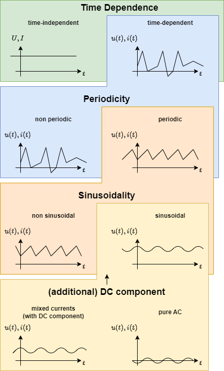
In the following we will investigate mainly pure AC signals.
6.2 Descriptive Values of AC Signals
Goals
After this lesson, you should:
- Know the relationship between amplitude and peak-to-peak value.
- Know the relationship between period, frequency and angular frequency.
- Know the difference between zero phase angle and phase shift angle.
- Know the direction of the phase shift angle.
- know the formula symbols of the above-mentioned quantities.
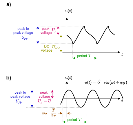
There are some important characteristic values when investigating AC signals (figure 2). For the singal itself these are:
- The DC voltage or DC offset is given by the value $U_{DC}$ of $V_{DC}$ (in German: Gleichanteil). The DC component also defines the average value of an AC signal.
- The maximum deviation from the DC value is called peak voltage $U_p$ (in German : Spitzespannung). Specifically for sinusidal signals the peak voltage $U_p$ is also called amplitude $\hat{U}$ (in German: Scheitelwert or Amplitude).
- The voltage difference between maximum and minimum deviation is called peak-to-peak voltage $U_{pp}$ (in German: Spitze-Spitze-Spannung).
Be aware, that in English texts often amplitude is also used for (non sinusidal) $U_{pp}$ - based on German DIN standards the term amplitude is only valid for the sinusidal peak voltage.
Additionally, there are also characteristic values related to the time:
- The shortest time difference for the signal to repeat is called period $T$.
- Based on the period $T$ the frequency $f = {{1}\over{T}}$ can be derived. The unit of the frequency is $1 Hz = 1 Hertz$.
- For calculation, often the angular frequency $\omega$ is used. The angular frequency is given by $\omega = {{2\pi}\over{T}}$ with the unit ${{1}\over{s}}$.
The angular frequency represents the angle which is covered in one second. - Another handy value is the time offset between the start of the sinus wave ($u(t)=0V$ and rising) and $t=0s$. This difference is often written based on an angular difference and is called the phase angle or initial phase $\varphi_U$ (in German: Nullphasenwinkel). This then has to be calculated back to a time value: $\Delta t= {{\varphi_U}\over{\omega}}= \varphi_U\cdot{{T}\over{2\pi}}$
Mathematically, the AC voltages and currents can be written as:
$$u(t)=\hat{U}\cdot sin(\omega t + \varphi_U)$$
$$i(t)=\hat{I}\cdot sin(\omega t + \varphi_I)$$
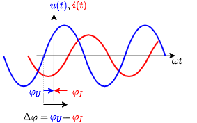
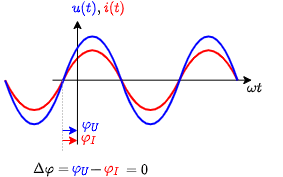
Between the AC voltages and currents there is also another important characteristic: The phase difference $\Delta \varphi$ is given by $\Delta \varphi = \varphi_U + \varphi_I$. The phase difference shows how far the momentary value of the current is ahead of the momentary value of the voltage.
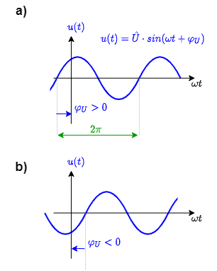
Notice:
The initial phase $\varphi_0$ has an direction / sign which have to be considered. In the case a) in the picture the zero-crossing of the sinusidal signal is before $t=0$ or $\omega t =0$. Therefore, the initial phase $\varphi_0$ is positive.
Similarly also for the phase difference $\Delta \varphi$ the direction has to be taken into account. In the following image the zero-crossing of the voltage curve is before the zero-crossing of the current. This leads to a positive phase difference $\Delta \varphi$.
6.3 AC Two-Poles
Goals
After this lesson, you should:
- know that real, lossy components are described by equivalent circuits of ideal components.
- know and be able to apply the definition of apparent resistance, apparent conductance, impedance, and admittance.
In the chapters 2. Simple Circuits and 3 Non-ideal Sources and Two Pole Networks we already have seen, that it is possible to reduce complex circuitries down to equivalent resistors (and ideal sources). This we will try to adopt for AC components, too.
We want to analyze
Resistance
We start with Ohms law, which states, that the instantaneous voltage $u(t)$ is proportional to the instantaneous current $i(t)$ by the factor $R$. $$u(t) = R \cdot i(t)$$
Then we insert the functions representing the instantaneous signals: $x(t)= \sqrt{2}{X}\cdot sin(\omega t + \varphi_x)$: $$\sqrt{2}{U}\cdot sin(\omega t + \varphi_u) = R \cdot \sqrt{2}{I}\cdot sin(\omega t + \varphi_i)$$
Since we know, that $u(t)$ must be proportional to $i(t)$ we conclude that for a resistor $\varphi_u=\varphi_i$!
\begin{align*} R &= {{\sqrt{2}{I}\cdot sin(\omega t + \varphi_i)}\over{\sqrt{2}{U}\cdot sin(\omega t + \varphi_i) }} \\ &= {{U}\over{I}} \end{align*}
This was not too hard und quite obvious. But, what about the other types of passive two-poles - namely the capacitance and inductance?
Capacitance
For the capacitance we have the principle formula: $$C={{Q}\over{U}}$$ This formula ia also true for the instantaneous values: $$C={{q(t)}\over{u(t)}}$$ Additionally we know, that the instantaneous current is defined by $i(t)={{dq(t)}\over{dt}}$.
By this we can set up the formula: \begin{align*} i(t) &= {{dq(t)}\over{dt}} \\ &= {{d}\over{dt}}\left( C \cdot u(t) \right) \end{align*}
Now, we insert the functions representing the instantaneous signals and calculate the derivative: \begin{align*} \sqrt{2}{I}\cdot sin(\omega t + \varphi_i) &= {{d}\over{dt}}\left( C \cdot \sqrt{2}{U}\cdot sin(\omega t + \varphi_u) \right) \\ &= C \cdot \sqrt{2}{U}\cdot \omega \cdot cos(\omega t + \varphi_u) \\ \\ {I}\cdot sin(\omega t + \varphi_i) &= C \cdot {U}\cdot \omega \cdot sin(\omega t + \varphi_u + {{1}\over{2}}\pi) \tag{6.3.1} \end{align*}
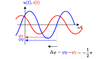
Equating coefficients in $(6.3.1)$ leads to: \begin{align*} I &= C \cdot U \cdot \omega \\ {{U}\over{I}} &= {{1}\over{\omega \cdot C}} \end{align*} and: \begin{align*} \omega t + \varphi_i &= \omega t + \varphi_u + {{1}\over{2}}\pi \\ \varphi_i &= \varphi_u + {{1}\over{2}}\pi \\ \varphi_u -\varphi_i &= - {{1}\over{2}}\pi \end{align*}
The phase shift of $- {{1}\over{2}}\pi$ can also be seen in figure 6 and figure 5.
Notice:
In order not to mix up the definitions, for AC signals the fraction of rms voltage by rms current is called apparent impedance $Z$ (in German: Scheinwiderstand or Impedanz).The apparent impedance is generally defined as $$Z = {{U}\over{I}}$$
Only for pure resistor two pole the apparent impedance $Z_R$ is equal to the value of the restance: $Z_R=R$.
Inductance
The inductance will here be introduced shortly - the detailed introduction is part of electrical engineering 2.
For the capacitance $C$ we had the situation, that it reacts to a voltage change ${{d}\over{dt}}u(t)$ with a counteracting current:
$$i(t)= C \cdot {{d}\over{dt}}u(t)$$
This is due to the fact, that the capacity stores charge carriers $q$. It appears that “the capacitance does not like voltage changes and reacts with a compensating current”. When the voltage on a capacity drops it supplies a current, when the voltage rises it drains a current.
For an inductance $L$ it is just the other way around: “the inductance does not like current changes and reacts with a compensating voltage drop”. Once the current changes it will create a voltage drop that counteracts and continues the current: A current change ${{d}\over{dt}}i(t)$ lead to a voltage drop $u(t)$: $$u(t)= L \cdot {{d}\over{dt}}i(t)$$ The proportionality factor here is the value of the inductance $L$ and it is measured in $[L] = 1H = 1\; Henry$.
We can now again insert the functions representing the instantaneous signals and calculate the derivative: \begin{align*} \sqrt{2}{U}\cdot sin(\omega t + \varphi_u) &= L \cdot {{d}\over{dt}}\left( \sqrt{2}{I}\cdot sin(\omega t + \varphi_i) \right) \\ &= L \cdot \sqrt{2}{I}\cdot \omega \cdot cos(\omega t + \varphi_i) \\ \\ {U}\cdot sin(\omega t + \varphi_u) &= L \cdot {I}\cdot \omega \cdot sin(\omega t + \varphi_i + {{1}\over{2}}\pi) \tag{6.3.2} \end{align*}
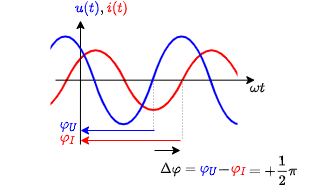
Equating coefficients in $(6.3.2)$ leads to: \begin{align*} U &= L \cdot {I}\cdot \omega \\ \boxed{Z_L = {{U}\over{I}} = \omega \cdot L} \end{align*} and: \begin{align*} \omega t + \varphi_u &= \omega t + \varphi_i + {{1}\over{2}}\pi \\ \varphi_u &= \varphi_i + {{1}\over{2}}\pi \\ \boxed{\varphi = \varphi_u -\varphi_i = + {{1}\over{2}}\pi } \end{align*}
The phase shift of $+ {{1}\over{2}}\pi$ can also be seen in figure 8 and figure 7.
Notice:
Remember the formulas for the different pure loads:| Load | apparent impedance $Z={{U}\over{I}}$ | phase $\varphi$ | |
|---|---|---|---|
| Resistance | $R$ | $Z_R = R $ | $\varphi_R = 0$ |
| Capacitance | $C$ | $Z_C = {{1}\over{\omega \cdot C}} $ | $\varphi_C = - {{1}\over{2}}\pi $ |
| Impedance | $L$ | $Z_L = \omega \cdot L $ | $\varphi_L = + {{1}\over{2}}\pi $ |
One way to memorize the phase shift is given bei the word CIVIL:
- CIVIL: for a capacitance C the current I leads the voltage V.
Therefore the phase angle $\varphi_I$ of the current is larger than the phase angle $\varphi_U$ of the voltage: $\rightarrow \varphi = \varphi_U - \varphi_I < 0 $. - CIVIL: for an inductance L the voltage V leads the current I.
Therefore the phase angle $\varphi_U$ of the voltge is larger than the phase angle $\varphi_I$ of the current: $\rightarrow \varphi = \varphi_U - \varphi_I > 0 $.
By the concept of AC two-poles we are also able to use the DC methods of network analysis in order to solve AC networks.
6.4 Complex Impedance
Goals
After this lesson, you should:
- know how sine variables can be symbolized by a vector.
- know which parameters can determine a sinusoidal quantity.
- be able to graphically derive a pointer diagram for several existing sine variables.
- be able to plot the phase shift on the vector and time plots.
- Be able to add sinusoidal quantities in vector and time representation.
- know and be able to apply the impedance of components.
- know the frequency dependence of the impedance of the components. In particular, you should know the effect of the ideal components at very high and very low frequencies and be able to apply it for plausibility checks.
Up to now, we used for the AC signals the formula $x(t)= {{1}\over{\sqrt{2}}} X \cdot sin (\omega t + \varphi_x)$ - which was quite obvious.
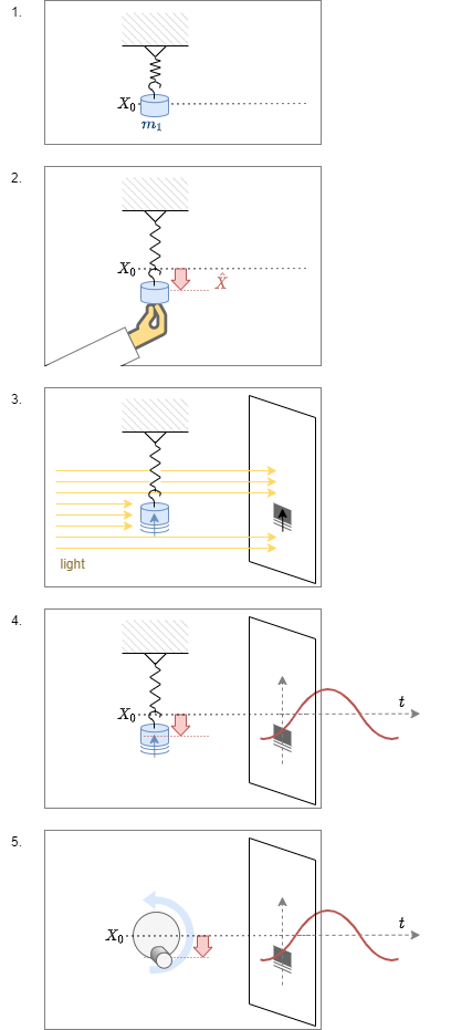
However, there is an alternative way to look onto the alternating sinusidal signals. For this, we look first on a different, but already familiar problem (see figure 9).
- A mechanical, linear spring with the characteristic constant $D$ is displaced due a mass $m$ in the Earth's gravitational field. The deflection only based on the gravitational field is $X_0$.
- At the time $t_0=0$ , we deflect this spring a bit more to $X_0 + x(t_0)=X_0 + \hat{X}$ and therefore induce energy into the system.
- When the mass is released, the mass will spring up and down for $t>0$. The signal can be shown as shadow when the mass is illuminated sideways.
For $t>0$, the energy is continuously shifted between poential energy (deflection $x(t)$ around $X_0$) and kinetic energy (${{d}\over{dt}}x(t)$) - When looking onto the course of time of $x(t)$, the signal will behave as: $x(t)= \hat{X} \cdot sin (\omega t + \varphi_x)$
- The movement of the shadow can also be created by a the sideways shadow of a stick on a rotating disc.
This means, that a two dimensional rotation is reduced down to a single dimension.
The transformation of the two dimensional rotation to a one dimensional sinusidal signal is also shown in figure 10.
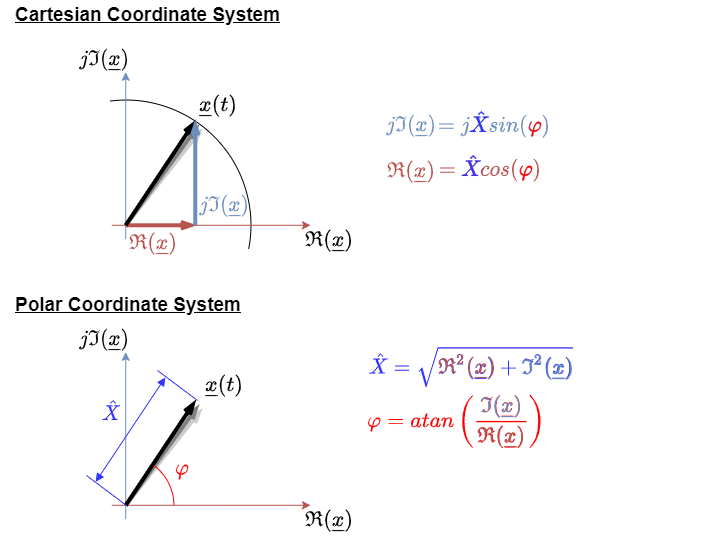
The two dimensional rotation can be represented with a complex number in Euler's formula. It combines the exponential representation with real part $\Re$ and imaginary part $\Im$ of a complex value: $$ \underline{x}(t)=\hat{X}\cdot e^{j(\omega t + \varphi_x)} = \Re(\underline{x}) + j\cdot \Im(\underline{x})$$
For the imaginary unit $i$ the letter $j$ is used in electical engineering, since the letter $i$ is already taken for currents.
6.6 Complex AC Impedance
Goals
After this lesson you should:
- Be able to draw and read pointer diagrams.
- Know and be able to apply the complex value formulas of impedance, reactance, resistance.
Video
Pointer diagrams; complex alternating current calculus.
Complex alternating current calculation - basic terms: Impedance, Reactance, Resistance
Capacitor and inductance as complex resistors; pointer diagram
detailed explanation of impedances
Exercises
Video
Parallel connection of complex resistors / impedances
Why can a circuit with impedances only act purely ohmic?
more complex exam task: complex circuit I
more complex exam task: complex circuit II
Examination task: complex circuit III