This is an old revision of the document!
5. Inductances in Circuits
5.1 Basic Circuits
Focus here: uncoupled inductors!
5.1.1 Series Circuits
Based on $L = {{ \Psi(t)}\over{i}}$ and Kirchhoff's mesh law ($i=const$) the series circuit of inductions can be interpreted as a single current $i$ which generates multiple linked fluxes $\Psi$. Since the current must stay constant in the series circuit, the following applies for the equivalent inductor of a series connection of signle ones:
\begin{align*} L_{eq} &= {{\sum_i \Psi_i}\over{I}} = \sum_i L_i \end{align*}
A similar result can be derived from the induced voltage $u_{ind}= - L {{di}\over{dt}}$, when taking the situation of a series circuit (i.e. $i_1 = i_2 = i_1 = ... = i_{eq}$ and $u_{eq}= u_1 + u_2 + ...$):
\begin{align*} & u_{eq} & = &u_1 &+ &u_2 &+ ... \\ & - L_{eq} {{di_{eq} }\over{dt}} & = &- L_{1} {{di_{1} }\over{dt}} &- &L_{2} {{di_{2} }\over{dt}} &- ... \\ & L_{eq} {{di }\over{dt}} & = &L_{1} {{di }\over{dt}} &+ &L_{2} {{di }\over{dt}} &+ ... \\ & L_{eq} & = &L_{1} &+ &L_{2} &+ ... \\ \end{align*}
5.1.2 Parallel Circuits
For parallel circuits one can also start with the principles based on Kirchhoff's mesh law:
\begin{align*} u_{eq}= u_1 = u_2 = ... \\ \end{align*}
and Kirchhoff's nodal law:
\begin{align*} i_{eq}= i_1 + i_2 + ... \\ \end{align*}
Here, the formula for the induced voltage has to be rearranged:
\begin{align*} u_{ind} &= - L {{di}\over{dt}} \quad \quad | \int()dt \\ \int u_{ind} dt &= - L \cdot i \\ i &= - {{1}\over{L}} \cdot \int u_{ind} dt \\ \end{align*}
By this, we get:
\begin{align*} i_{eq} &=& i_1 &+& i_2 &+& ... \\ - {{1}\over{L_{eq}}} \cdot \int u_{eq} dt &=& - {{1}\over{L_1}} \cdot \int u_{1} dt &+& - {{1}\over{L_2}} \cdot \int u_{2} dt &+& ... \\ - {{1}\over{L_{eq}}} \cdot \int u dt &=& - {{1}\over{L_1}} \cdot \int u dt &+& - {{1}\over{L_2}} \cdot \int u dt &+& ... \\ {{1}\over{L_{eq}}} &=& {{1}\over{L_1}} &+& {{1}\over{L_2}} &+& ... \\ \end{align*}
Notice:
The inductor behaves in the parallel and series circuit similar to the resistor.5.1.3 in AC Circuits
For AC circuits (i.e. with sinosidal signals) the impedance $Z$ based on the real part $R$ and imaginary part $X$ has to be considered. In order to do so, one has to solve:
\begin{align*} \underline{Z} = {{\underline{u}}\over{\underline{i}}} \end{align*}
With the induction $u_{ind}= - L {{di}\over{dt}}$ we get:
\begin{align*} \underline{Z} = {{- L {{d\underline{i}}\over{dt}} }\over{\underline{i}}} \end{align*}
Without limiting the generality one can assume the current $i$ to be: $i = I \cdot \sqrt{2} \cdot e^{j \cdot \omega t + \varphi_0}$.
Therefore:
\begin{align*} \underline{Z} &= {{- L {{d I \cdot \sqrt{2} \cdot e^{j \cdot \omega t + \varphi_0}}\over{dt}}}\over{I \cdot \sqrt{2} \cdot e^{j \cdot \omega t + \varphi_0}}} \\ &= {{- L {{d}\over{dt}} I \cdot \sqrt{2} \cdot e^{j \cdot \omega t + \varphi_0}}\over{I \cdot \sqrt{2} \cdot e^{j \cdot \omega t + \varphi_0}}} \\ &= {{- L \cdot I \cdot \sqrt{2} \cdot {{d}\over{dt}}e^{j \cdot \omega t + \varphi_0}}\over{I \cdot \sqrt{2} \cdot e^{j \cdot \omega t + \varphi_0}}} \\ &= {{- L \cdot j \cdot \omega t \cdot e^{j \cdot \omega t + \varphi_0}}\over{e^{j \cdot \omega t + \varphi_0}}} \\ &= - L \cdot j \cdot \omega t \\ \end{align*}
5.2 Charging and Discharging
- signal time course
- comparison with RC-circuit chraging / discharging
5.3 Resonance Phenomena
Link to: consideration on sinusidal signals in EE1
5.3.1 RLC - Series Resonant Circuit
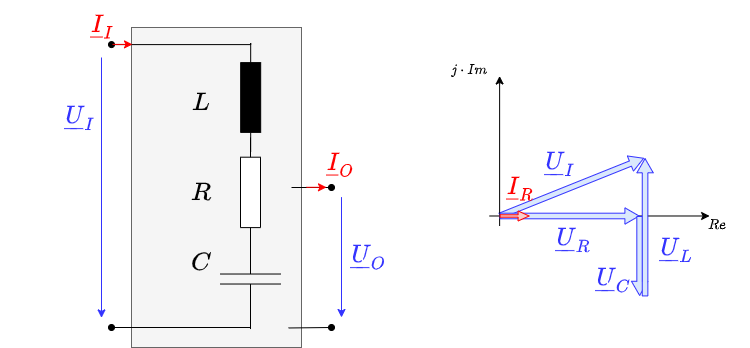
If a resistor $R$, a capacitor $C$ and an inductance $L$ are connected in series, the result is a series resonant circuit. In this case the output voltage is not clearly defined. It must be considered in the following how the voltages behave across the individual components. The total voltage (= input voltage $U_I$) results to:
\begin{align*} \underline{U} = \underline{U}_R + \underline{U}_L + \underline{U}_C \end{align*}
Since the current in the circuit must be constant, the total impedance can be determined here in a simple way:
\begin{align*} \underline{U} &= R \cdot \underline{I} + j \omega L \cdot \underline{I} + \frac {1}{j\omega C } \cdot \underline{I} \\ \underline{U} &= \left( R + j \omega L - j \cdot \frac {1}{\omega C } \right) \cdot \underline{I}\\ \underline{Z}_{ges} &= R + j \omega L - j \cdot \frac {1}{\omega C } \end{align*}
As the magnitude of the (input) voltage $U$ or the (input or total) impedance $Z$ and the phase result to:
\begin{align*} U &= \sqrt{U_R^2 + (U_Z)^2} = \sqrt{U_R^2 + (U_L - U_C)^2} \end{align*}
\begin{align*} Z &= \sqrt{R^2 + (Z)^2} = \sqrt{R^2 + (\omega L - \frac{1}{\omega C})^2} \end{align*}
\begin{align*} \varphi_u = \varphi_Z &= arctan \frac{\omega L - \frac{1}{\omega C}}{R} \end{align*}
There are now 3 different situations to distinguish:
- If $U_L > U_C$ the whole setup behaves like an ohmic-inductive load. This is the case at high frequencies.
- If $U_L$ equals $U_C$, the total input voltage $U$ is applied to the resistor. In this case, the total resistance $Z$ is minimal and only ohmic.
Thus, the current $I$ is then maximal. If the current is maximum, then the responses of the capacitance and inductance - their voltages - are also maximum. This situation is the resonance case. - If $U_L < U_C$ then the whole setup behaves like a resistive-capacitive load. This is the case at low frequencies.
Again, there seems to be an excellent frequency, namely when $U_L = U_C$ or $Z_C = Z_L$ holds:
\begin{align*} \frac{1}{\omega_0 C} & = \omega L \\ \omega_0 & = \frac{1}{\sqrt{LC}}\\ 2\pi f_0 & = \frac{1}{\sqrt{LC}} \rightarrow \boxed{ f_0 = \frac{1}{2\pi \sqrt{LC}} } \end{align*}
The frequency $f_0$ is called resonance frequency.
| $\quad$ | $f \rightarrow 0$ | $\quad$ | $f = f_0$ | $\quad$ | $f \rightarrow \infty$ | |
|---|---|---|---|---|---|---|
| voltage $U_R$ at the resistor | $\boldsymbol{0}$ | $\boldsymbol{U}$ since the impedances just cancel | $ \boldsymbol{0}$ | |||
| voltage $U_L$ at the inductor | $\boldsymbol{0}$ because $\omega L$ becomes very small | $\boldsymbol{\omega_0 L \cdot I = \omega_0 L \cdot \frac{U}{R} = \color{blue}{\frac{1}{R}\sqrt{\frac{L}{C}}\cdot U}}$ | $\boldsymbol{U}$ since $\omega L$ becomes very large |
|||
| $\boldsymbol{U}$ \voltage $U_C$ at the capacitor | $\boldsymbol{U}$ because $\frac{1}{\omega C}$ becomes very large | $\boldsymbol{\frac{1}{\omega_0 C} \cdot I = \frac{1}{\omega_0 C} \cdot \frac{U}{R} = \color{blue}{\frac{1}{R}\sqrt{\frac{L}{C}}\cdot U}}$ | $\boldsymbol{0}$ \because $\frac{1}{\omega C}$ becomes very small |
The calculation in the table shows that in the resonance case, the voltage across the capacitor or inductor deviates from the input voltage by a factor $\color{blue}{\frac{1}{R}\sqrt{\frac{L}{C}}}$. This quantity is called quality or Q-factor $Q_S$:
\begin{align*} \boxed{ Q_S = \frac{U_C}{U} |_{\omega = \omega_0} = \frac{U_L}{U} |_{\omega = \omega_0} = \color{blue}{\frac{1}{R}\sqrt{\frac{L}{C}}} } \end{align*}
The quality can be greater than, less than or equal to 1.
- If the quality is very high, the overshoot of the voltages at the impedances becomes very large in the resonance case. This is useful and necessary in various applications, e.g. in an RLC element as an antenna.
- If the Q is very small, overshoot is no longer seen. Depending on the impedance at which the output voltage is measured, a high-pass or low-pass is formed similar to the RC or RL element. However, this has a steeper slope in the blocking range. This means that the filter effect is better.
The reciprocal of the Q is called attenuation $d_S$. This is specified when using the circuit as a non-overshooting filter.
\begin{align*} \boxed{ d_S = \frac{1}{Q_S} = R \sqrt{\frac{C}{L}} } \end{align*}
5.4 Applications of Inductors
- ferrite bead
- Decoupling
- Filter
- unwanted coupling and cirucit design
5.x Examples
Decoupling capacitor on the microcontroller
Simulation in Falstad. Note: The simulation gives a highly simplified picture. The response of the microcontroller is shown reduced to a triangular signal, since the slope of the voltages cannot be represented. A real simulation requires a powerful SPICE program in which the conduction theory can be represented.
Further details can be found here (practice), here (layout), also Layout or Layout.