1 The Electrostatic Field
- Chapter 5. Electric Charges and Fields
- Chapter 6. Gauss's Law
- Chapter 7. Electrical Potential
- Chapter 8. Capacitance
Every day life teaches us that there are various charges and their effects. The image figure 1 depicts a chargeable body that can be charged through charge separation between the sole and the floor. The movement of the foot generates a negative surplus charge in the body, which progressively spreads throughout the body. A current can flow even through the air if a pointed portion of the body (e.g., a finger) is brought into close proximity to a charge reservoir with no extra charges.
We had already considered the charge as the central quantity of electricity in the first chapter of the previous semester and recognized it as a multiple of the elementary charge. There was already a mutual force action (the Coulomb-force) derived. This will be more fully explained.
First, we shall define certain terms:
- Electricity is a catch-all term for any occurrences involving moving and resting charges.
- Electrostatics is the study of charges at rest and consequently electric fields that do not vary over time. As a result, the electrical quantities have no temporal dependence.
For any function of the electric quantities, ${{{\rm d} f}\over{{\rm d} t}}=0$ holds mathematically. - Electrodynamics describes the behavior of moving charges. Hence, electrodynamics covers both changing electric fields and magnetic fields.
For the time being, the simple explanation will be that magnetic fields are dependent on current or charge flow.
It is no longer true in electrodynamics that the derivative is always necessary for any function of electric values.
Only electrostatics is discussed in this chapter. For the time being, magnetic fields are thus excluded. Furthermore, electrodynamics is not covered in this chapter and is provided in further detail in subsequent chapters.
1.1 Electric Field and Field Lines
Learning Objectives
By the end of this section, you will be able to:
- Know that an electric field is formed around a charge.
- Sketch the field lines of electric fields.
- Represent the field vectors in a sketch when given several charges.
- Determine the resulting field vector by superimposing several field vectors using vector calculus.
- Determine the force on a charge in an electrostatic field by applying Coulomb's law. Specifically:
- The force vector in coordinate representation
- The magnitude of the force vector
- The angle of the force vector
educational Task
The simulation was already mentioned briefly in the first chapter. However, another issue must be addressed here.
Place a negative charge $Q$ in the middle of the simulation and turn off the electric field. The latter is accomplished by using the hook on the right. The situation is now close to reality because a charge appears to have no effect at first glance.
A sample charge $q$ is placed near the existing charge $Q$ for impact analysis (in the simulation, the sample charge is called “sensors”). The charge $Q$ is observed to affect a force on the sample charge. At any point in space, the magnitude and direction of this force can be determined. In space, the force behaves similarly to gravity. A field serves to describe the condition space changed by the charge $Q$.
Fig. 2: setup for own experiments
Take a charge ($+1~{ \rm nC}$) and position it.
Measure the field across a sample charge (a sensor).
The concept of a field will now be briefly discussed in more detail.
- The introduction of the field distinguishes the cause from the effect.
- The field in space is caused by the charge $Q$.
- As a result of the field, the charge $q$ in space feels a force.
- This distinction is brought up again in this chapter.
It is also fairly obvious in electrodynamics at high frequencies: the field corresponds to photons, i.e. to a transmission of effects with a finite (light)speed $c$.
- There are different-dimensional fields, just like physical quantities:
- In a scalar field, each point in space is assigned a single number.
For example,- a temperature field $T(\vec{x})$ on a weather map or in an object
- a pressure field $p(\vec{x})$
- Each point in space in a vector field is assigned several numbers in the form of a vector. This reflects the action as it occurs along the spatial coordinates.
As an example.- gravitational field $\vec{g}(\vec{x})$ pointing to the object's center of mass.
- electric field $\vec{E}(\vec{x})$
- magnetic field $\vec{H}(\vec{x})$
- A tensor field is one in which each point in space is associated with a two- or more-dimensional physical quantity - that is, a tensor. Tensor fields are useful in mechanics (for example, the stress tensor), but they are not required in electrical engineering.
Vector fields are defined as follows:
- Effects along spatial axes $x$, $y$ and $z$ (Cartesian coordinate system).
- Effect in magnitude and direction vector (polar coordinate system)
Note:
- Fields describe a physical state of space.
- Here, a physical quantity is assigned to each point in space.
- The electrostatic field is described by a vector field.
The Electric Field
To determine the electric field, a measurement of its magnitude and direction is now required. The Coulomb force between two charges $Q_1$ and $Q_2$ is known from the first chapter of the previous semester:
\begin{align*} F_C = {{{1} \over {4\pi\cdot\varepsilon}} \cdot {{Q_1 \cdot Q_2} \over {r^2}}} \end{align*}
The force on a (fictitious) sample charge $q$ is now considered to obtain a measure of the magnitude of the electric field.
\begin{align*} F_C &= {{{1} \over {4\pi\cdot\varepsilon}} \cdot {{Q_1 \cdot q} \over {r^2}}} \\ &= \underbrace{{{1} \over {4\pi\cdot\varepsilon}} \cdot {{Q_1} \over {r^2}}}_\text{=independent of q} \cdot q \\ \end{align*}
As a result, the left part is a measure of the magnitude of the field, independent of the size of the sample charge $q$. Thus, the magnitude of the electric field is given by
$E = {{1} \over {4\pi\cdot\varepsilon}} \cdot {{Q_1} \over {r^2}} \quad$ with $[E]={{[F]}\over{[q]}}=1 ~{ \rm {N}\over{As}}=1 ~{ \rm {N\cdot m}\over{As \cdot m}} = 1 ~{ \rm {V \cdot A \cdot s}\over{As \cdot m}} = 1 ~{ \rm {V}\over{m}}$
The result is therefore \begin{align*} \boxed{F_C = E \cdot q} \end{align*}
Note:
- The test charge $q$ is always considered to be positive (mnemonic: t = +). It is only used as a thought experiment and has no retroactive effect on the sampled charge $Q$.
- The sampled charge here is always a point charge.
Note:
At a measuring point $P$, a charge $Q$ produces an electric field $\vec{E}(Q)$. This electric field is given by- the magnitude $|\vec{E}|=\Bigl| {{1} \over {4\pi\cdot\varepsilon}} \cdot {{Q_1} \over {r^2}} \Bigl| $ and
- the direction of the force $\vec{F_C}$ experienced by a sample charge on the measurement point $P$. This direction is indicated by the unit vector $\vec{e_{ \rm r}}={{\vec{F_C}}\over{|F_C|}}$ in that direction.
Be aware that in English courses and literature $\vec{E} $ is simply referred to as the electric field, and the electric field strength is the magnitude $|\vec{E}|$. In German notation, the Elektrische Feldstärke refers to $\vec{E}$ (magnitude and direction), and the Elektrische Feld denotes the general presence of an electrostatic interaction (often without considering exact magnitude).
The direction of the electric field is switchable in figure 2 via the “Electric Field” option on the right.
The electric field can also be viewed again in this video.
Electric Field Lines
Electric field lines result from the (fictitious) path of a sample charge. Thus, also electric field lines of several charges can be determined. However, these also result from a superposition of the individual effects - i.e., electric field - at a measuring point $P$.
The superposition is sketched in figure 3: Two charges $Q_1$ and $Q_2$ act on the test charge $q$ with the forces $F_1$ and $F_2$. Depending on the positions and charges, the forces vary, and so does the resulting force. The simulation also shows a single field line.
For a full picture of the field lines between charges, one has to start with a single charge. The in- and outgoing lines on this charge are drawn equidistant from the charge. This is also true for the situation with multiple charges. However, there, the lines are not necessarily run radially anymore. The test charge is influenced by all the single charges, and therefore, the field lines can get bent.

In figure 5 the field lines are shown. The additional “equipotential lines” will be discussed later and can be deactivated by clearing the checkmark Show Equipotentials.
Try the following in the simulation:
- Get accustomed to the simulation. You can…
- … move the charges by drag and drop.
- … add another Charge with
Add»Add Point Charge. - … delete components with a right click on them and
delete
- Where is the density of the field lines higher?
- How does the field between two positive charges look? How does it look between two different charges?
Note:
- The electrostatic field is a source field. This means there are sources and sinks.
- From the field line diagrams, the following can be obtained:
- Direction of the field ($\hat{=}$ parallel to the field line).
- Magnitude of the field ($\hat{=}$ number of field lines per unit area).
- The magnitude of the field along a field line is usually not constant.
Note:
Field lines have the following properties:- The electric field lines have a beginning (at a positive charge) and an end (at a negative charge).
- The direction of the field lines represents the direction of a force onto a positive test charge.
- There are no closed field lines in electrostatic fields. The reason for this can be explained by considering the energy of the moved particle (see later subchapters).
- Electric field lines cannot cut each other: This is based on the fact that the direction of the force at a cutting point would not be unique.
- The field lines are always perpendicular to conducting surfaces. This is also based on energy considerations; more details later.
- The inside of a conducting component is always field-free. Also, this will be discussed in the following.
Tasks
Task 1.1.1 simple task with charges
Task 1.1.2 Field lines

1.2 Electric Charge and Coulomb Force (reloaded)
Learning Objectives
By the end of this section, you will be able to:
- Determine the direction of the forces using the given charges.
- Represent the acting force vectors in a sketch.
- Determine a force vector by superimposing several force vectors using vector calculus.
- State the following quantities for a force vector:
- The force vector in coordinate representation
- The magnitude of the force vector
- The angle of the force vector
The electric charge and Coulomb force have already been described last semester. However, some points are to be caught up here.
Direction of the Coulomb force and Superposition
In the case of the force, only the direction has been considered so far, e.g., direction towards the sample charge. For future explanations, it is important to include the cause and effect in the naming. This is done by giving the correct labeling of the subscript of the force. In figure 7 (a) and (b), the convention is shown: A force $\vec{F}_{21}$ acts on charge $Q_2$ and is caused by charge $Q_1$. As a mnemonic, you can remember “tip-to-tail” (first the effect, then the cause).
Furthermore, several forces on a charge can be superimposed, resulting in a single, equivalent force.
Strictly speaking, it must hold that $\varepsilon$ is constant in the structure. For example, the resultant force in figure 7 Fig. (c) on $Q_3$ becomes equal to: $\vec{F_3}= \vec{F_{31}}+\vec{F_{32}}$.
Fig. 7: direction of coulomb force
.

Geometric Distribution of Charges
In previous chapters, only single charges (e.g., $Q_1$, $Q_2$) were considered.
- The charge $Q$ was previously reduced to a point charge.
This can be used, for example, for the elementary charge or for extended charged objects from a large distance. The distance is sufficiently large if the ratio between the largest object extent and the distance to the measurement point $P$ is small. - If the charges are lined up along a line, this is referred to as a line charge.
Examples of this are a straight trace on a circuit board or a piece of wire. Furthermore, this also applies to an extended charged object, which has exactly an extension that is no longer small in relation to the distance. For this purpose, the charge $Q$ is considered to be distributed over the line. Thus, a (line) charge density $\rho_l$ can be determined:$\rho_l = {{Q}\over{l}}$
or, in the case of different charge densities on subsections:
$\rho_l = {{\Delta Q}\over{\Delta l}} \rightarrow \rho_l(l)={{\rm d}\over{{\rm d}l}} Q(l)$
- It is spoken of as an area charge when the charge is distributed over an area.
Examples of this are the floor or the plate of a capacitor. Again, an extended charged object can be considered when two dimensions are no longer small in relation to the distance (e.g. surface of the earth). Again, a (surface) charge density $\rho_A$ can be determined:$\rho_A = {{Q}\over{A}}$
or if there are different charge densities on partial surfaces:
$\rho_A = {{\Delta Q}\over{\Delta A}} \rightarrow \rho_A(A) ={{\rm d}\over{{\rm d}A}} Q(A)={{\rm d}\over{{\rm d}x}}{{\rm d}\over{{\rm d}y}} Q(A)$
- Finally, a space charge is the term for charges that span a volume.
Here, examples are plasmas or charges in extended objects (e.g., the doped volumes in a semiconductor). As with the other charge distributions, a (space) charge density $\rho_V$ can be calculated here:$\rho_V = {{Q}\over{V}}$
or for different charge density in partial volumes:
$\rho_V = {{\Delta Q}\over{\Delta V}} \rightarrow \rho_V(V) ={{\rm d}\over{{\rm d}V}} Q(V)={{\rm d}\over{{\rm d}x}}{{\rm d}\over{{\rm d}y}}{{\rm d}\over{{\rm d}z}} Q(V)$
In the following, area charges and their interactions will be considered.
Types of Fields depending on the Charge Distribution
There are two different types of fields:
In homogeneous fields, magnitude and direction are constant throughout the field range. This field form is idealized to exist within plate capacitors. e.g., in the plate capacitor (figure 9), or the vicinity of widely extended bodies.

For inhomogeneous fields, the magnitude and/or direction of the electric field changes from place to place. This is the rule in real systems, even the field of a point charge is inhomogeneous (figure 10).

Tasks
Task 1.2.1 Multiple Forces on a Charge I (exam task, ca 8% of a 60-minute exam, WS2020)

Given is the arrangement of electric charges in the picture on the right.
The following force effects result:
$F_{01}=-5 ~\rm{N}$
$F_{02}=-6 ~\rm{N}$
$F_{03}=+3 ~\rm{N}$
Calculate the magnitude of the resulting force.
- How have the forces be prepared, to add them correctly?
The forces have to be resolved into coordinates. Here, it is recommended to use an orthogonal coordinate system ($x$ and $y$).
The coordinate system shall be in such a way, that the origin lies in $Q_0$, the x-axis is directed towards $Q_3$ and the y-axis is orthogonal to it.
For the resolution of the coordinates, it is necessary to get the angles $\alpha_{0n}$ of the forces with respect to the x-axis.
In the chosen coordinate system this leads to: $\alpha_{0n} = \arctan(\frac{\Delta y}{\Delta x})$
$\alpha_{01} = \arctan(\frac{3}{1})= 1.249 = 71.6°$
$\alpha_{02} = \arctan(\frac{4}{3})= 0.927 = 53.1°$
$\alpha_{03} = \arctan(\frac{0}{3})= 0= 0°$
Consequently, the resolved forces are:
\begin{align*} F_{x,0} &= F_{x,01} + F_{x,02} + F_{x,03} && | \quad \text{with } F_{x,0n} = F_{0n} \cdot \cos(\alpha_{0n}) \\ F_{x,0} &= (-5~\rm{N}) \cdot \cos(71.6°) + (-6~\rm{N}) \cdot \cos(53.1°) + (+3~\rm{N}) \cdot \cos(0°) \\ F_{x,0} &= -9.54 ~\rm{N} \\ \\ F_{y,0} &= F_{y,01} + F_{y,02} + F_{y,03} && | \quad \text{with } F_{y,0n} = F_{0n} \cdot \sin(\alpha_{0n}) \\ F_{y,0} &= (-5~\rm{N}) \cdot \sin(71.6°) + (-6~\rm{N}) \cdot \sin(53.1°) + (+3~\rm{N}) \cdot \sin(0°) \\ F_{y,0} &= -2.18 ~\rm{N} \\ \\ \end{align*}
Task 1.2.2 Variation: Multiple Forces on a Charge II (exam task, ca 8% of a 60 minute exam, WS2020)

Given is the arrangement of electric charges in the picture on the right.
The following force effects result:
$F_{01}=-5 ~\rm{N}$
$F_{02}=-6 ~\rm{N}$
$F_{03}=+3 ~\rm{N}$
Calculate the magnitude of the resulting force.
Task 1.2.3 Variation: Multiple Forces on a Charge II (exam task, ca 8% of a 60 minute exam, WS2020)

Given is the arrangement of electric charges in the picture on the right.
The following force effects result:
$F_{01}=+2 ~\rm{N}$
$F_{02}=-3 ~\rm{N}$
$F_{03}=+4 ~\rm{N}$
Calculate the magnitude of the resulting force.
Task 1.2.4 Superposition of Charges in 1D
1.3 Work and Potential
Learning Objectives
By the end of this section, you will be able to:
- Know how work is defined in the electrostatic field.
- Describe when work has to be performed and when it does not in the situation of a movement.
- Know the definition of electric voltage and be able to calculate it in an electric field.
- Understand why the calculation of voltage is independent of displacement.
- Know what a potential difference is and recognize or be able to state equipotential surfaces (lines).
- Determine a potential curve for a given arrangement.
A detailed explanation can be found in the online book 'University Physics II'. It is recommended to work through this independently.
In particular, this applies to:
- Chapter “7. electric potential”
Energy required to Displace a Charge in the electric Field
First, the situation of a charge in a homogeneous electric field shall be considered. As we have seen so far, the magnitude of $E$ is constant, and the field lines are parallel. Now, a positive charge $q$ is to be brought into this field.
If this charge were free movable (e.g., an electron in a vacuum or an extended conductor), it would be accelerated along field lines. Thus, its kinetic energy increases. Because the whole system of plates (for field generation) and charge, however, does not change its energetic state, thermodynamically, the system is closed. From this follows: if the kinetic energy increases, the potential energy must decrease.
Fig. 11: Observation of work in a homogeneous electric field

It is known from mechanics that the work done (thus the energy needed) is defined by the force one needs to move along a path.
In a homogeneous field, the following holds for a force-producing motion along a field line from ${ \rm A}$ to ${ \rm B}$ (see figure 11):
\begin{align*}
W_{ \rm AB} = F_C \cdot s
\end{align*}
For a motion perpendicular to the field lines (i.e. from ${ \rm A}$ to ${ \rm C}$) no work is needed - so $W_{ \rm AC}=0$ results - because the formula above is only true for $F_C$ parallel to $s$. The motion perpendicular to the field lines is similar to the movement of weight in the gravitational field at the same height. Or more illustratively: It is similar to walking on the same floor of a house. There, too, no energy is released or absorbed concerning the field. For any direction through the field, the part of the path has to be considered, which is parallel to the field lines. This results from the angle $\alpha$ between $\vec{F}$ and $\vec{s}$: \begin{align*} W_{\rm AB} = F_C \cdot s \cdot \cos(\alpha) = \vec{F_C}\cdot \vec{s} \end{align*}
The work $W_{ \rm AB}$ here describes the energy difference experienced by the charge $q$.
Similar to the electric field, we now look for a quantity that is independent of the (sample) charge $q$ to describe the energy component. This is done by the voltage $U$. The voltage of a movement from $A$ to $B$ in a homogeneous field is defined as:
\begin{align} U_{ \rm AB} = {{W_{ \rm AB}}\over{q}} = {{F_C \cdot s}\over{q}} = {{E \cdot q \cdot s}\over{q}} = E \cdot s_{ \rm AB} \end{align}
Note:
- The voltage $U_{ \rm AB}$ represents the work $W$ per charge needed to move a probe charge from point $A$ to point {B} in an $E$-field.
- The voltage is measured in Volts: $[U] = 1~{ \rm V}$
To obtain a general approach to inhomogeneous fields and arbitrary paths $s_{ \rm AB}$, it helps (as is so often the case) to decompose the problem into small parts. In the concrete case, these are small path segments on which the field can be assumed to be homogeneous. These are to be assumed to be infinitesimally small in the extreme case (i.e., from $s$ to $\Delta s$ to $ds$):
\begin{align} W_{ \rm AB} = \vec{F_C}\cdot \vec{s} \quad \rightarrow \quad \Delta W = \vec{F_C}\cdot \Delta \vec{s}\quad \rightarrow \quad {\rm d}W = \vec{F_C}\cdot {\rm d} \vec{s} \end{align}
The total energy now results from the sum or integration of these path sections:
\begin{align*} W_{ \rm AB} &= \int_{W_{ \rm A}}^{W_{ \rm B}} {\rm d} W \ &= \int_{ \rm A}^{ \rm B} \vec{F_C}\cdot {\rm d} \vec{s} \\ &= \int_{ \rm A}^{ \rm B} q \cdot \vec{E} \cdot {\rm d} \vec{s} \\ &= q \cdot \int_{ \rm A}^{ \rm B} \vec{E} \cdot {\rm d} \vec{s} \end{align*}
The voltage is therewith:
\begin{align*} U_{ \rm AB} &= {{W_{ \rm AB}}\over{q}} &= \int_{ \rm A}^{ \rm B} \vec{E} \cdot {\rm d} \vec{s} \end{align*}
Interestingly, it does not matter which way the integration takes place. So, it doesn't matter how the charge gets from ${ \rm A}$ to ${ \rm B}$: the energy needed and the voltage are always the same. This follows from the fact that a charge $q$ at a point ${ \rm A}$ in the field has a unique potential energy. No matter how this charge is moved to a point ${ \rm B}$ and back again: as soon as it gets back to point ${ \rm A}$, it has the same energy again. So the voltage of the way there and back must be equal in magnitude.
Fig. 12: different Paths in a Field

This independence of the taken path leads to the closed path in figure 12 from ${ \rm A}$ to ${ \rm B}$ and back to:
\begin{align*} \sum W &= W_{ \rm AB} &+ W_{ \rm BA} \\ &= q \cdot U_{ \rm AB} &+ q \cdot U_{ \rm BA} \\ &= q \cdot (U_{ \rm AB} + U_{ \rm BA} ) = 0 \end{align*}
Therefore:
\begin{align*} U_{ \rm AB} + U_{ \rm BA} &= 0 \\ \int_{ \rm A}^{ \rm B} \vec{E} \cdot {\rm d} \vec{s} + \int_{ \rm B}^{ \rm A} \vec{E} \cdot {\rm d} \vec{s} &= 0 \\ \rightarrow \boxed{ \oint \vec{E} \cdot {\rm d} \vec{s} = 0} \end{align*}
This concept has already been applied as Kirchhoff's voltage law (mesh theorem) in circuits (see prevoius semester). However, it is also valid in other structures and arbitrary electrostatic fields.
Note:
- Returning to the starting point from any point $A$ after a closed circuit, the circuit voltage along the closed path is 0.
A closed path is mathematically expressed as a ring integral: \begin{align} U = \oint \vec{E} \cdot {\rm d} \vec{s} = 0 \end{align} - Or spoken differently: In the electrostatic field, there are no self-contained field lines.
- A field $\vec{X}$ which satisfies the condition $\oint \vec{X} \cdot {\rm d} \vec{s}=0$ is referred to as vortex-free or potential field.
From the potential difference, or the voltage, the work in the electrostatic field results as: \begin{align*} \boxed{W_{ \rm AB}= q \cdot U_{ \rm AB}} \end{align*}
Equipotential Lines

In the previous subchapter, the term voltage got a more general meaning. This shall now be applied to investigate the electric field a bit more. Once a charge $q$ moves perpendicular to the field lines, it experiences neither energy gain nor loss. The voltage along this path is $0~{ \rm V}$. All points where the voltage of $0~{ \rm V}$ is applied are at the same potential level. The connection of these points is referred to as:
- equipotential lines for a 2-dimensional representation of the field.
- equipotential surfaces for a 3-dimensional field
This corresponds in the gravity field to a movement on the same contour line. The contour lines are often drawn in (hiking) maps, cf. figure 13. If one moves along the contour lines, no work is done.
In figure 14, the equipotential lines of a point charge are shown.
- The equipotential surfaces are drawn with a fixed step size, e.g. $1~{ \rm V}$, $2~{ \rm V}$, $3~{ \rm V}$, ….
- Since the electric field is higher near charges, equipotential surfaces are also closer together there.
- The angle between the field vectors (and therefore the field lines) and the equipotential lines is always $90°$
Electric Potential
So up to now, the voltage was investigated, and also equipotential areas were found. But what is this potential anyway? Since the voltage is independent of the path, one can conclude that the path integral can always be expressed as the difference between two scalar values:
\begin{align*} U_{ \rm AB} &= \int_{ \rm A}^{ \rm B} \vec{E} \cdot {\rm d} \vec{s} \\ &= \varphi_{ \rm A} - \varphi_{ \rm B} \end{align*}

Here, the electric potential $\varphi$ is introduced as the scalar local function of the electric field (see figure 15). This means: any point in space can either be connected to the two-dimensional value $\vec{E}$ or the one-dimensional value $\varphi$. Both fully and equally represent the electrostatic field.
Similar to the reference or ground level for the altitude in the gravitational field, the reference or ground potential can be chosen arbitrarily for a single task. Often, the ground potential $\varphi_{ \rm G}= \varphi_{ \rm GND}$ is chosen to be located at infinity (see figure 16). In this case, the potential at the point $\rm A$ can be calculated as follows:
Fig. 16: electric Potential at Infinity

\begin{align*} U_{ \rm AB} &= \int_{ \rm A}^{ \rm B} \vec{E} \cdot {\rm d} \vec{s} &= \varphi_{ \rm A} - \varphi_{ \rm B} \\ \rightarrow U_{ \rm AZ} &= \int_{ \rm A}^{ \rm Z} \vec{E} \cdot {\rm d} \vec{s} &= \varphi_{ \rm A} - \underbrace{\varphi_{ \rm Z}}_\text{=0} \\ \\ \rightarrow \varphi_{ \rm A} &= \int_{ \rm A}^{\infty} \vec{E} \cdot {\rm d} \vec{s} \end{align*}
Alternatively, also the potential $\varphi_{ \rm B}$ could also be considered as ground potential. This would lead to the following potentials for $\varphi_{ \rm A}$ and $\varphi_{ \rm C}$:
\begin{align*} \varphi_{ \rm A} &= \varphi_{ \rm A} - \underbrace{\varphi_{ \rm B}}_\text{=0} \\ &= \int_{ \rm A}^{ \rm B} \vec{E} \cdot {\rm d} \vec{s} \end{align*}
\begin{align*} \varphi_{ \rm C} &= \varphi_{ \rm C} - \underbrace{\varphi_{ \rm B}}_\text{=0} \\ &= \int_{ \rm C}^{ \rm B} \vec{E} \cdot {\rm d} \vec{s} \\ &= - \int_{ \rm B}^{ \rm C} \vec{E} \cdot {\rm d} \vec{s} \\ \end{align*}
For a positive charge the potential nearby, the charge is positive and increasing, the closer one gets (see figure 17).
Application of the electric Potential
The equation $U_{ \rm AB} = \int_{ \rm A}^{ \rm B} \vec{E} \cdot {\rm d} \vec{s}$ can be used and applied depending on the geometry present. As an example, consider the situation of a charge moving from one electrode to another inside a capacitor:\begin{align*} U_{ \rm AB} &= \int_{ \rm A}^{ \rm B} \vec{E} \cdot {\rm d} \vec{s} \quad && | \vec{E} \text{ and } {\rm d}\vec{s} \text{ run parallel } \\ U_{ \rm AB} &= \int_{ \rm A}^{ \rm B} E \cdot {\rm d}s \quad && | \text{E = const.} \\ U_{ \rm AB} &= E \cdot \int_{0}^{d} {\rm d}s \quad && | s \text{ starts at the negative plate. } d \text{ denotes the distance between the two plates }\\ U &= E \cdot d \quad && | U_{ \rm AB} \text{ corresponds to the voltage applied to the capacitor } U \\ \end{align*}
1.4 Conductors in the Electrostatic Field
Learning Objectives
By the end of this section, you will be able to:
- Know that no current flows in a conductor in an electrostatic field.
- Know how charges in a conductor are distributed in the electrostatic field.
- Sketch the field lines at the surface of the conductor.
- Understand the effect of the electrostatic induction of an external electric field.
Up to now, charges were considered that were either rigid or not freely movable. In the following, charges on an electric conductor are investigated. These charges are only free to move within the conductor. At first, an ideal conductor without resistance is considered.
Stationary Situation of a charged Object without an external Field
In the first thought experiment, a conductor (e.g., a metal plate) is charged, see figure 18.
The additional charges create an electric field. Thus, a resultant force acts on each charge.
The causes of this force are the electric fields of the surrounding electric charges. So the charges repel and move apart.
Fig. 18: Viewing a charged metal ball

The movement of the charge continues until a force equilibrium is reached.
In this steady state, there is no longer a resultant force acting on the single charge.
In figure 18 this can be seen on the right: the repulsive forces of the charges are counteracted by the attractive forces of the atomic shells.
Results:
- The charge carriers are distributed on the surface.
- Due to the dispersion of the charges, the interior of the conductor is free of fields.
- All field lines are perpendicular to the surface. Because: if they were not, there would be a parallel component of the field, i.e., along the surface. Thus, a force would act on charge carriers, and they would move accordingly.
Educational Task - Why is there a discharge at pointy ends of conductors?
Point discharge is a well-known phenomenon, which can be seen as corona discharge on power lines (where it also creates the summing sound) or is used in spark plugs. The phenomenon addresses the effect that there are many more charges at the corners and edges of a conductor. But why is that so? For this, it is feasible to try to calculate the charge density at different spots of a conductor.

In the figure 20 an example of a “pointy” conductor is given in image (a). The surface of the conductor is always at the same potential. To cope with this complex shape and the desired charge density, the following path shall be taken:
- It is good to first calculate the potential field of a point charge.
For this calculate $U_{ \rm CG} = \int_{ \rm C}^{ \rm G} \vec{E} \cdot {\rm d} \vec{s}$ with $\vec{E} ={{1} \over {4\pi\cdot\varepsilon}} \cdot {{q} \over {r^2}} \cdot \vec{e}_r $, where $\vec{e}_r$ is the unit vector pointing radially away, ${ \rm C}$ is a point at distance $r_0$ from the charge and ${ \rm G}$ is the ground potential at infinity. - Compare the field and the potentials of the different spherical conductors in figure 20, image (b).
- Are there differences for the electric field $\vec{E}$ outside the spherical conductors? Are the potentials on the surface the same?
- What can be conducted for the field of the three situations in (b) and (d), when the total charge on the surface is considered to be always the same?
- For spherical conductors, the surface charge density is constant. Given that this charge density leads to the overall charge $q$, how does $\varrho_A$ depend on the radius $r$ of a sphere?
- Now, the situation in (c) shall be considered. Here, all components are conducting, i.e., the potentials on the surface are similar. Both spheres shall be considered to be as far away from each other, so that they show an undisturbed field near their surfaces. In this case, charges on the surface of the curvature to the left and the right represent the same situation as in (a). For the next step, it is important that by this, the potentials of the left sphere with $q_1$ and $r_1$ and the right sphere with $q_2$ and $r_2$ are the same.
- Set up this equality formula based on the formula for the potential from question 1.
- Insert the relationship for the overall charges $q_1$ and $q_2$ based on the surface charge densities $\varrho_{A1}$ and $\varrho_{A2}$ of a sphere and their radii $r_1$ and $r_2$.
- What is the relationship between the bending of the surface and the charge density?
Electrostatic Induction
In the second thought experiment, an uncharged conductor (e.g., a metal plate) is brought into an electrostatic field (figure 21).
The external field or the resulting Coulomb force causes the moving charge carriers to be displaced.
Fig. 21: Viewing the induced charge separation

Results:
- The charge carriers are still distributed on the surface.
- Now, equilibrium is reached when just so many charges have moved, that the electric field inside the conductor disappears (again).
- The field lines leave the surface again at right angles. Again, a parallel component would cause a charge shift in the metal.
This effect of charge displacement in conductive objects by an electrostatic field is referred to as electrostatic induction (in German: Influenz). Induced charges can be separated (figure 21 right). If we look at the separated induced charges without the external field, their field is again just as strong in magnitude as the external field only in the opposite direction.
Note:
- The location of an induced charge is always on the conductor surface. This results in a surface charge density $\varrho_A = {{\Delta Q}\over{\Delta A}}$
- The conductor surface in the electrostatic field is always an equipotential surface. Thus, the field lines always originate and terminate perpendicularly on conductor surfaces.
- The interior of the conductor is always field-free (Faraday effect: metallic enclosures shield electric fields).
How can the conductor surface be an equipotential surface despite different charges on both sides? Equipotential surfaces are defined only by the fact that the movement of a charge along such a surface does not require/produce a change in energy. Since the interior of the conductor is field-free, movement there can occur without a change in energy. As the potential between two points is independent of the path between them, a path along the surface is also possible without energy expenditure.
Tasks
Application of electrostatic induction: Protective bag against electrostatic charge/discharge (cf. Video)
Task 1.4.1 Simulation
In the simulation in figure 23, the equipotential lines and electric field at different objects can be represented. In the beginning, the situation of an infinitely long cylinder in a homogeneous electric field is shown. The solid lines show the equipotential surfaces. The small arrows show the electric field.
- What is the angle between the field on the surface of the cylinder?
- Once the option
Flat Viewis deactivated, an alternative view of this situation can be seen. Additionally, charged test particles can be added withDisplay: Particles (Vel.). This alternative view looks similar to what other physical fields? - What can be said about the potential distribution on the cylinder?
- On the left half of the field lines enter the body, on the right half, they leave the body. What can be said about the charge carrier distribution at the surface? Check also the representation
Floor: charge! - Is there an electric field inside the body?
- Is this cylinder metallic, semiconducting, or insulating?
Task 1.4.5 Simulation
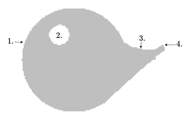
Given is the two-dimensional component shown in figure 24. The component shall be charged positively.
In the picture, there are 4 positions marked with numbers.
Order the numbered positions by increasing charge density!
1.5 The Electric Displacement Field and Gauss's Law of electrostatics
Learning Objectives
By the end of this section, you will be able to:
- Know how to get the electric displacement field from single charges
- State for a given area the electric displacement field of an arrangement
- Know the general meaning of Gauss's law of electrostatics
- Choose a closed surface appropriately and apply Gauss's law
For a detailed description please see the chapters 6.2 Electric Flux and 6.3 Explaining Gauss's Law.
Electric Displacement Flux Density D
Up to now, …
- … we investigated the effect of the electric field onto a (probe) charge, which can be calculated by $\vec{F}= \vec{E}\cdot q$.
- … the field $\vec{E}$ is principally a property of the space and the charges inside it.
- … we also only had a look at “empty space” containing charges and/or ideally conducting components
The following introduced electric displacement flux density $\vec{D}$ is only focusing on the cause of the electric fields. The effect can differ since the space can also “hinder” the electric field in an effect. This is especially true when the situation within a material and not a vacuum has to be analyzed.
To investigate this situation, we want to consider two conductive plates (X) and (Y) with the area $\Delta A$ in the electrostatic field $\vec{E}$ in a vacuum, a little more exactly. For this purpose, the plates shall first be brought into the field separately.
Fig. 26: induced charge separation and electric displacement field

As written in figure 26 a), the electrostatic induction in a single plate is not considered. Rather, we are now interested in what happens based on the electrostatic induction when the plates are brought together. The electrostatic induction will again move charges inside the conductors. Near the negative outer plate (1), positive charges get induced on (X). Equally, near to positive outer plate (2), negative charges get induced on (Y). Graphically speaking, for each field line ending on the pair of plates, a single charge must move from one plate to the other. The direction of the movement is similar to the direction of $\vec{E}$. This ability to separate charges (i.e,. to generate electrostatic induction) is another property of space. This property is independent of any matter inside the space.
This movement is represented by the displacement flux $\Psi$. The displacement flux is given by the amount of moved charge $\Psi = n \cdot e = Q$, with the unit $[\Psi]= [Q] = 1~{ \rm C}$. When looking at figure 26 b) and c), it is evident that for larger plates (X) and (Y) more charges get displaced. So, to get a constant value by dividing the displacement flux by the corresponding area. This leads to the electric displacement field $D$ (sometimes also displacement flux density), which is defined as:
\begin{align*} \boxed{ D = {{\Psi}\over{A}} } \end{align*}
On the other hand one could also only focus on the induced charges on the surfaces: In the shown arrangement (homogeneous field, all surfaces parallel to each other), the surface charge density $\varrho_A = {{\Delta Q}\over{\Delta A}}$ thus electrostatic induction is proportional to the external field $E$. It holds:
\begin{align*} \varrho_A = {{\Delta Q}\over{\Delta A}} \sim E \\ \varrho_A = {{\Delta Q}\over{\Delta A}} = \varepsilon \cdot E \end{align*}
Since the induced charges $\Delta Q$ are equal to the flux $\Psi$ the electric displacement field is also given by:
\begin{align} \boxed{\vec{D} = \varepsilon \cdot \vec{E}} \end{align}
- Similar to the electric field $\vec{E}$ also the flux density is a field.
- It can be interpreted as a vector field. pointing in the same direction as the electric field $\vec{E}$.
- The electric displacement field has the unit “charge per area”, i.e. ${ \rm As/m^2}$.
Why is a second field introduced? This shall become clearer in the following, but first, it shall be considered again how the electric field $\vec{E}$ was defined. This resulted from the Coulomb force, i.e., the action on a sample charge. The electric displacement field, on the other hand, is not described by an action, but caused by charges. The two are related by the above equation. It will be shown in later sub-chapters that the different influences from the same cause of the field can produce different effects on other charges.
The permittivity (or dielectric conductivity) $\varepsilon$ thus results as a constant of proportionality between $D$-field and $E$-field. The inverse ${{1}\over{\varepsilon}}$ is a measure of how much effect ($E$-field) is available from the cause ($D$-field) at a point. In a vacuum, $\varepsilon$ is $\varepsilon_0$, the electric field constant.
General relationship between Charge Q and electric Displacement Field D
Up to now, only a homogeneous field was considered, and only a surface perpendicular to the field lines. Thus, only equipotential surfaces (e.g., a metal foil) were investigated. In that case, it was found that the charge is equal to the electric displacement field on the surface: $\Delta Q = D\cdot \Delta A$.
This formula is now to be extended to arbitrary surfaces and inhomogeneous fields. As with the potential and other physical problems, the problem is to be broken down into smaller sub-problems, solved, and then summed up. For this purpose, a small area element $\Delta A = \Delta x \cdot \Delta y$ is needed. In addition, the position of the area in space should be taken into account. This is possible if the cross product is chosen: $\Delta \vec{A} = \Delta \vec{x} \times \Delta \vec{y}$, since so is the surface normal. In what follows, the cross-product will be relevant to the calculation, but the consequences of the cross-product will be:
- The magnitude of $\Delta \vec{A}$ is equal to the area $\Delta A$.
- The direction of $\Delta \vec{A}$ is perpendicular to the area.
In addition, let $\Delta A$ now become infinitesimally small, that is, ${\rm d}A = {\rm d}x \cdot {\rm d}y$.
1. Problem: Inhomogenity → Solution: infinitesimal Area
First, we shall still assume an observation surface perpendicular to the field lines, but an inhomogeneous field. In the inhomogeneous field, the magnitude of $D$ is no longer constant. To correct this, ${\rm d}A$ is chosen so small that just “only one field line” passes through the surface. In this case, $D$ is homogeneous again. Thus holds:
$Q = D\cdot A$
\begin{align*} Q = D\cdot A \quad \rightarrow \quad {\rm d}Q = D\cdot {\rm d}A \end{align*}

2nd problem: arbitrary surface → solution: vectors
Now, assume an arbitrary surface. Thus, the $\vec{D}$-field no longer penetrates through the surface at right angles. But for the electrostatic induction, only the rectangular part was relevant. So only this part has to be considered. This results from consideration of the cosine of the angle between (right-angled) area vector and $\vec{D}$-field:
\begin{align*} {\rm d}Q = D\cdot {\rm d}A \quad \rightarrow \quad {\rm d}Q = D\cdot {\rm d}A \cdot \cos(\alpha) = \vec{D} \cdot {\rm d} \vec{A} \end{align*}

The area vector and the surface normal can be seen in figure 29.

3. Summing up
Since so far only infinitesimally small surface pieces have been considered must now be integrated again into a total surface. If a closed enveloping surface around a body is chosen, the result is:
\begin{align} \boxed{\int {\rm d}Q = {\rlap{\rlap{\int_A} \int} \: \LARGE \circ} \vec{D} \cdot {\rm d} \vec{A} = \iiint_V \varrho_V {\rm d}\vec{V} = Q} \end{align}
The symbol ${\rlap{\Large \rlap{\int} \int} \, \LARGE \circ}$ denotes that there is a closed surface used for the integration.
The “sum” of the $D$-field emanating over the surface is thus just as large as the sum of the charges contained therein, since the charges are just the sources of this field. This can be compared with a bordered swamp area with water sources and sinks:
- The sources in the marsh correspond to the positive charges, and the sinks to the negative charges. The formed water corresponds to the $D$-field.
- The sum of all sources and sinks equals, in this case, just the water stepping over the edge.

Applications
They are calculated in the course.
Spherical Capacitor
Spherical capacitors are now rarely found in practical applications. In the Van-de-Graaff generator, spherical capacitors are used to store the high DC voltages. The earth also represents a spherical capacitor. In this context, the electric field of $100...300~{ \rm V/m}$ in the atmosphere is remarkable since several hundred volts would have to be present between head and foot (for resolution, see the article Electricity from the air in Bild der Wissenschaft).
Plate Capacitor
The relation between the $E$-field and the voltage $U$ on the ideal plate capacitor is to be derived from the integral of displacement flux density $\vec{D}$: \begin{align*} Q = {\rlap{\rlap{\int_A} \int} \: \LARGE \circ} \vec{D} \cdot {\rm d} \vec{A} \end{align*}
Outlook
The consideration of the displacement flux density also solved a problem that arose for electric series circuits. We know that the current at each point of a series circuit is the same. But what if there is a capacitor in this series circuit? There is no electric current flowing inside the dielectric material. This problem can be solved considering the connection of magnetic fields and current flow: any magnetic field is based on a moving charge, and any moving charge creates a magnetic field. By this, the solution is that the temporal change of the displacement flux is interpreted as a current, which is generated by a magnetic field (thus a magnetic “vortex” around the circuit). Mathematically, vortices are described via the Curl (in German: Rotation) - a multidimensional differential operator. A deeper derivation and solution is not considered in the first semester. However, the application will show that the equation above plays a central role in electrical engineering. It is part of the so-called Maxwell's equations.tasks
Task 1.5.1 induced Charges
A plate capacitor with a distance of $d = 2 ~{ \rm cm}$ between the plates and with air as dielectric ($\varepsilon_{ \rm r}=1$) gets charged up to $U = 5~{ \rm kV}$. In between the plates, a thin metal foil with the area $A = 45~{ \rm cm^2}$ is introduced parallel to the plates.
Calculate the amount of the displaced charges in the thin metal foil.
- What is the strength of the electric field $E$ in the capacitor?
- Calculate the displacement flux density $D$
- How can the charge $Q$ be derived from $D$?
Task 1.5.2 Manipulating a Capacitor I
An ideal plate capacitor with a distance of $d_0 = 7 ~{ \rm mm}$ between the plates gets charged up to $U_0 = 190~{ \rm V}$ by an external source. The source gets disconnected. After this, the distance between the plates gets enlarged to $d_1 = 7 ~{ \rm cm}$.
- What happens to the electric field and the voltage?
- How does the situation change (electric field/voltage), when the source is not disconnected?
- Consider the displacement flux through a surface around a plate
- $U_1 = 1.9~{ \rm kV}$, $E_1 = 27~{ \rm kV/m}$
- $U_1 = 190~{ \rm V}$, $E_1 = 2.7~{ \rm kV/m}$
Task 1.5.3 Manipulating a Capacitor II
An ideal plate capacitor with a distance of $d_0 = 6 ~{ \rm mm}$ between the plates and with air as dielectric ($\varepsilon_0=1$) is charged to a voltage of $U_0 = 5~{ \rm kV}$. The source remains connected to the capacitor. In the air gap between the plates, a glass plate with $d_{ \rm g} = 4 ~{ \rm mm}$ and $\varepsilon_{ \rm r} = 8$ is introduced parallel to the capacitor plates.
1. Calculate the partial voltages on the glas $U_{ \rm g}$ and on the air gap $U_{ \rm a}$.
- Build a formula for the sum of the voltages first
- How is the voltage related to the electric field of a capacitor?
The sum of the voltages across the glass and the air gap gives the total voltage $U_0$, and each individual voltage is given by the $E$-field in the individual material by $E = {{U}\over{d}}$: \begin{align*} U_0 &= U_{\rm g} + U_{\rm a} \\ &= E_{\rm g} \cdot d_{\rm g} + E_{\rm a} \cdot d_{\rm a} \end{align*}
The displacement field $D$ must be continuous across the different materials since it is only based on the charge $Q$ on the plates. \begin{align*} D_{\rm g} &= D_{\rm a} \\ \varepsilon_0 \varepsilon_{\rm r, g} \cdot E_{\rm g} &= \varepsilon_0 \cdot E_{\rm a} \end{align*}
Therefore, we can put $E_\rm a= \varepsilon_{\rm r, g} \cdot E_\rm g $ into the formula of the total voltage and rearrange to get $E_\rm g$: \begin{align*} U_0 &= E_{\rm g} \cdot d_{\rm g} + \varepsilon_{\rm r, g} \cdot E_{\rm g} \cdot d_{\rm a} \\ &= E_{\rm g} \cdot ( d_{\rm g} + \varepsilon_{\rm r, g} \cdot d_{\rm a}) \\ \rightarrow E_{\rm g} &= {{U_0}\over{d_{\rm g} + \varepsilon_{\rm r, g} \cdot d_{\rm a}}} \end{align*}
Since we know that the distance of the air gap is $d_{\rm a} = d_0 - d_{\rm a}$ we can calculate: \begin{align*} E_{\rm g} &= {{5'000 ~\rm V}\over{0.004 ~{\rm m} + 8 \cdot 0.002 ~{\rm m}}} \\ &= 250 ~\rm{{kV}\over{m}} \end{align*}
By this, the individual voltages can be calculated: \begin{align*} U_{ \rm g} &= E_{\rm g} \cdot d_\rm g &&= 250 ~\rm{{kV}\over{m}} \cdot 0.004~\rm m &= 1 ~{\rm kV}\\ U_{ \rm a} &= U_0 - U_{ \rm g} &&= 5 ~{\rm kV} - 1 ~{\rm kV} &= 4 ~{\rm kV}\\ \end{align*}
2. What would be the maximum allowed thickness of a glass plate, when the electric field in the air-gap shall not exceed $E_{ \rm max}=12~{ \rm kV/cm}$?
Now we shall eliminate $E_\rm g$, since $E_\rm a$ is given in the question. \begin{align*} U_0 &= E_{\rm g} \cdot d_{\rm g} + E_{\rm a} \cdot d_{\rm a} \\ &= {{E_\rm a}\over{\varepsilon_{\rm r,g}}} \cdot d_{\rm g} + E_{\rm a} \cdot d_{\rm a} \\ \end{align*}
The distance $d_\rm a$ for the air is given by the overall distance $d_0$ and the distance for glass $d_\rm g$: \begin{align*} d_{\rm a} = d_0 - d_{\rm g} \end{align*}
This results in: \begin{align*} U_0 &= {{E_{\rm a}}\over{\varepsilon_{\rm r,g}}} \cdot d_{\rm g} + E_{\rm a} \cdot (d_0 - d_{\rm g}) \\ {{U_0}\over{E_{\rm a} }} &= {{1}\over{\varepsilon_{\rm r,g}}} \cdot d_{\rm g} + d_0 - d_{\rm g} \\ &= d_{\rm g} \cdot ({{1}\over{\varepsilon_{\rm r,g}}} - 1) + d_0 \\ d_{\rm g} &= { { {{U_0}\over{E_{\rm a} }} - d_0 } \over { {{1}\over{\varepsilon_{\rm r,g}}} - 1 } } &= { { d_0 - {{U_0}\over{E_{\rm a} }} } \over { 1 - {{1}\over{\varepsilon_{\rm r,g}}} } } \end{align*}
With the given values: \begin{align*} d_{\rm g} &= { { 0.006 {~\rm m} - {{5 {~\rm kV} }\over{ 12 {~\rm kV/cm}}} } \over { 1 - {{1}\over{8}} } } &= { {{8}\over{7}} } \left( { 0.006 - {{5 }\over{ 1200}} } \right) {~\rm m} \end{align*}
Task 1.5.4 Spherical capacitor
Two concentric spherical conducting plates set up a spherical capacitor. The radius of the inner sphere is $r_{ \rm i} = 3~{ \rm mm}$, and the inner radius from the outer sphere is $r_{ \rm o} = 9~{ \rm mm}$.
- What is the capacity of this capacitor, given that air is used as a dielectric?
- What would be the limit value of the capacity when the inner radius of the outer sphere goes to infinity ($r_{ \rm o} \rightarrow \infty$)?
- What is the displacement flux density of the inner sphere?
- Out of this derive the strength of the electric field $E$
- What ist the general relationship between $U$ and $\vec{E}$? Derive from this the voltage between the spheres.
- $C = 0.5~{ \rm pF}$
- $C_{\infty} = 0.33~{ \rm pF}$
Task 1.5.5 Applying Gauss's law: Electric Field of a line charge
1.6 Non-Conductors in electrostatic Field
Learning Objectives
By the end of this section, you will be able to:
- Know the two field-describing quantities of the electrostatic field,
- Describe and apply the relationship between these two quantities via the material law,
- Understand the effect of an electrostatic field on an insulator,
- Know what the effect of dielectric polarization does,
- Relate the term dielectric strength to a property of insulators and know what it means
The material law of electrostatics
First of all, a thought experiment is to be carried out again (see figure 31):
- First, a charged plate capacitor in a vacuum is assumed, which is separated from the voltage source after charging.
- Next, the intermediate region is to be filled with a material.

Think about how $E$ and $D$ would change before you unfold the subsection.
Why might one of the two quantities change?
You may have considered what happens to the charge $Q$ on the plates. This charge cannot escape the plates. So $Q = {\rlap{\Large \rlap{\int_A} \int} \, \LARGE \circ} \enspace \vec{D} \cdot {\rm d} \vec{A}$ cannot change.
Since the fictitious surface around an electrode does not change either, $\vec{D}$ cannot change either.

On the other hand, polarizable materials in the capacitor can align themselves. This dampens the effective field. Maybe you remember what the “acting field” was: the $E$-field. So the $E$-field becomes smaller (see figure 32).
Previously:
\begin{align*} D = \varepsilon_0 \cdot E \end{align*}
The determined change is packed into the material constant $\varepsilon_{ \rm r}$. This gives the material law of electrostatics:
\begin{align*} \boxed{D = \varepsilon_{ \rm r} \cdot \varepsilon_0 \cdot E} \end{align*}
Since the charge $Q$ cannot vanish from the capacitor in this experimental setup and thus $D$ remains constant, the $E$ field must become smaller for $\varepsilon_{ \rm r} > 1$.
figure 32 is drawn here in a simplified way: the alignable molecules are evenly distributed over the material and are thus also evenly aligned. Accordingly, the E-field is uniformly attenuated.
Note:
- The material constant $\varepsilon_{ \rm r}$ is referred to as relative permittivity, relative permittivity, or dielectric constant.
- Relative permittivity is unitless and indicates how much the electric field decreases in the presence of a material for the same charge.
- The relative permittivity $\varepsilon_{ \rm r}$ is always greater than or equal to 1 for dielectrics (i.e., nonconductors).
- The relative permittivity depends on the polarizability of the material, i.e., the possibility of aligning the molecules in the field. Correspondingly, relative permittivity depends on the frequency and often direction and temperature.
Outlook
Suppose now the relative permittivity $\varepsilon_{ \rm r}$ depends on the possibility of aligning the molecules in the field. In that case, the following interesting relation arises: if frequencies are “caught”, at which the oscillation of the molecule can build up, the energy of the external field is absorbed by the molecule. This build-up is similar to the shattering of a wine glass at a suitable irradiated frequency and is referred to as resonance. Materials can be analyzed based on the resonance frequencies. These resonance frequencies are enormously high ($1 ~{ \rm GHz}$ to $1'000'000 ~{ \rm GHz}$) and in these frequencies, the $E$-field detaches from the conductor. This may sound strange, but it becomes a bit more illustrative with the resonant circuits in the next chapters. For here it is more than sufficient that in the range of $1'000'000 ~{ \rm GHz}$ is the visual light, which is obviously not bound to a conductor. But this also makes clear that the relative permittivity $\varepsilon_{ \rm r}$ for high frequencies also has to do with the absorption (and reflection) of electromagnetic waves.Some values of the relative permittivity $\varepsilon_{ \rm r}$ for dielectrics are given in table 1.
Dielectric strength of dielectrics
- The dielectrics act as insulators. The flow of current is therefore prevented
- The ability to insulate is dependent on the material.
- If a maximum electric field $E_0$ is exceeded, the insulating ability is eliminated.
- One says: The insulator breaks down. This means that above this electric field, a current can flow through the insulator.
- Examples are: Lightning in a thunderstorm, ignition spark, glow lamp in a phase tester
- The maximum electric field $E_0$ is referred to as dielectric strength (in German: Durchschlagfestigkeit or Durchbruchfeldstärke).
- $E_0$ depends on the material (see table 2), but also on other factors (temperature, humidity, …).
tasks
Task 1.6.1 Thought Experiment
Consider what would have happened if the plates had not been detached from the voltage source in the above thought experiment (figure 31).
1.7 Capacitors
Learning Objectives
By the end of this section, you will be able to:
- Know what a capacitor is and how capacitance is defined,
- Know the basic equations for calculating capacitance and be able to apply them,
- Imagine a plate capacitor and give examples of its use. You also have an idea of what a cylindrical or spherical capacitor looks like and what examples of its use there are,
- Know the characteristics of the E-field, D-field, and electric potential in the three types of capacitors presented here
Capacitor and Capacitance
- A capacitor is defined by the fact that there are two electrodes (= conductive areas), which are separated by a dielectric (= non-conductor).
- This makes it possible to build up an electric field in the capacitor without charge carriers moving through the dielectric.
- The characteristic of the capacitor is the capacitance $C$.
- In addition to the capacitance, every capacitor also has resistance and inductance. However, both of these are usually very small.
- Examples are
- the electrical component “capacitor”,
- an open switch,
- a wire to ground,
- a human being
$\rightarrow$ Thus, for any arrangement of two conductors separated by an insulating material, a capacitance can be specified.
The capacitance $C$ can be derived as follows:
- It is known that $U = \int \vec{E} {\rm d} \vec{s} = E \cdot l$ and hence $E= {{U}\over{l}}$ or $D= \varepsilon_0 \cdot \varepsilon_{ \rm r} \cdot {{U}\over{l}}$.
- Furthermore, ${\rlap{\Large \rlap{\int_A} \int} \, \LARGE \circ} \; \vec{D} \cdot {\rm d} \vec{A} = Q$ by the idealized form of the plate capacitor: $Q=D \cdot A$.
- Thus, the charge $Q$ is given by: \begin{align*} Q = \varepsilon_0 \cdot \varepsilon_{ \rm r} \cdot {{U}\over{l}} \cdot A \end{align*}
- This means that $Q \sim U$, given the geometry (i.e., $A$ and $d$) and the dielectric ($\varepsilon_{ \rm r} $).
- So it is reasonable to determine a proportionality factor ${{Q}\over{U}}$.
The capacitance $C$ of an idealized plate capacitor is defined as
\begin{align*} \boxed{C = \varepsilon_0 \cdot \varepsilon_{ \rm r} \cdot {{A}\over{l}} = {{Q}\over{U}}} \end{align*}
Some of the main results here are:
- The capacity can be increased by increasing the dielectric constant $\varepsilon_{ \rm r} $, given the the same geometry.
- As near together the plates are as higher the capacity will be.
- As larger the area as higher the capacity will be.
The background behind the dielectric constant $\varepsilon_{ \rm r} $ and the field is explained in the following video
This relationship can be examined in more detail in the following simulation:
- Capacitor lab
-
If the simulation is not displayed optimally, this link can be used.
The figure 33 shows the topology of the electric field inside a plate capacitor.
Designs and types of capacitors
To calculate the capacitance of different designs, the definition equations of $\vec{D}$ and $\vec{E}$ are used. This can be viewed in detail, e.g., in this video.
Based on the geometry, different equations result (see also figure 34).

| Shape of the Capacitor | Parameter | Equation for the Capacity |
|---|---|---|
| plate capacitor | area $A$ of plate distance $l$ between plates | \begin{align*}C = \varepsilon_0 \cdot \varepsilon_{ \rm r} \cdot {{A}\over{l}} \end{align*} |
| cylinder capacitor | radius of outer conductor $R_{ \rm o}$ radius of inner conductor $R_{ \rm i}$ length $l$ | \begin{align*}C = \varepsilon_0 \cdot \varepsilon_{ \rm r} \cdot 2\pi {{l}\over{{\rm ln} \left({{R_{ \rm o}}\over{R_{ \rm i}}}\right)}} \end{align*} |
| spherical capacitor | radius of outer spherical conductor $R_{ \rm o}$ radius of inner spherical conductor $R_{ \rm i}$ | \begin{align*}C = \varepsilon_0 \cdot \varepsilon_{ \rm r} \cdot 4 \pi {{R_{ \rm i} \cdot R_{ \rm o}}\over{R_{ \rm o} - R_{ \rm i}}} \end{align*} |

In figure 35 different designs of capacitors can be seen:
- rotary variable capacitor (also variable capacitor or trim capacitor).
- A variable capacitor consists of two sets of plates: a fixed set and a movable set (stator and rotor). These represent the two electrodes.
- The movable set can be rotated radially into the fixed set. This covers a certain area of $A$.
- The size of the area is increased by the number of plates. Nevertheless, only small capacities are possible because of the necessary distance.
- Air is usually used as the dielectric; occasionally, small plastic or ceramic plates are used to increase the dielectric constant.
-
- In the multilayer capacitor, there are again two electrodes. Here, too, the area $A$ (and thus the capacitance $C$) is multiplied by the finger-shaped interlocking.
- Ceramic is used here as the dielectric.
- The multilayer ceramic capacitor is also referred to as KerKo or MLCC.
- The variant shown in (2) is an SMD variant (surface mound device).
- Disk capacitor
- A ceramic is also used as a dielectric for the disk capacitor. This is positioned as a round disc between two electrodes.
- Disc capacitors are designed for higher voltages, but have a low capacitance (in the microfarad range).
- Electrolytic capacitor, in German also referred to as Elko for Elektrolytkondensator
- In electrolytic capacitors, the dielectric is an oxide layer formed on the metallic electrode. The second electrode is the liquid or solid electrolyte.
- Different metals can be used as the oxidized electrode, e.g., aluminum, tantalum, or niobium.
- Because the oxide layer is very thin, a very high capacitance results (depending on the size: up to a few millifarads).
- Important for the application is that it is a polarized capacitor. I.e., it may only be operated in one direction with DC voltage. Otherwise, a current can flow through the capacitor, which destroys it and is usually accompanied by an explosive expansion of the electrolyte. To avoid reverse polarity, the negative pole is marked with a dash.
- The electrolytic capacitor is built up wrapped, and often has a cross-shaped predetermined breaking point at the top for gas leakage.
- film capacitor, in German also referred to as Folko, for Folienkondensator.
- A material similar to a “chip bag” is used as an insulator: a plastic film with a thin, metalized layer.
- The construction shows a high pulse load capacitance and low internal ohmic losses.
- In the event of an electrical breakdown, the foil enables “self-healing”: the metal coating evaporates locally around the breakdown. Thus the short-circuit is canceled again.
- With some manufacturers, this type is referred to as MKS (Mmetallized foilccapacitor, Polyester).
- Supercapacitor (engl. Super-Caps)
- As a dielectric is - similar to the electrolytic capacitor - very thin. In the actual sense, there is no dielectric at all.
- The charges are not only stored in the electrode, but - similar to a battery - the charges are transferred into the electrolyte. Due to the polarization of the charges, they surround themselves with a thin (atomic) electrolyte layer. The charges then accumulate at the other electrode.
- Supercapacitors can achieve very large capacitance values (up to the Kilofarad range), but only have a low maximum voltage


In figure 34 are shown different capacitors:
- The above two SMD capacitors
- On the left a $100~{ \rm µF}$ electrolytic capacitor
- On the right a $100~{ \rm nF}$ MLCC in the commonly used Surface-mount_technology 0603 ($1.6~{ \rm mm}$ x $0.8~{ \rm mm}$)
- below different THT capacitors (Through Hole Technology)
- A big electrolytic capacitor with $10~{ \rm mF}$ in blue, the positive terminal is marked with $+$
- In the second row is a Kerko with $33~{ \rm pF}$ and two Folkos with $1,5~{ \rm µF}$ each
- In the bottom row, you can see a trim capacitor with about $30~{ \rm pF}$ and a tantalum electrolytic capacitor and another electrolytic capacitor
Various conventions have been established for designating the capacitance value of a capacitor various conventions.
Electrolytic capacitors can explode!
Note:
- There are polarized capacitors. With these, the installation direction and current flow must be observed, as otherwise, an explosion can occur.
- Depending on the application - and the required size, dielectric strength, and capacitance - different types of capacitors are used.
- The calculation of the capacitance is usually not via $C = \varepsilon_0 \cdot \varepsilon_{ \rm r} \cdot {{A}\over{l}} $ . The capacitance value is given.
- The capacitance value often varies by more than $\pm 10~{ \rm \%}$. I.e., a calculation accurate to several decimal places is rarely necessary/possible.
- The charge current seems to be able to flow through the capacitor because the charges added to one side induce correspondingly opposite charges on the other side.
1.8 Circuits with Capacitors
Learning Objectives
By the end of this section, you will be able to:
- Recognize a series connection of capacitors and distinguish it from a parallel connection,
- Calculate the resulting total capacitance of a series or parallel circuit,
- Know how the total charge is distributed among the individual capacitors in a parallel circuit,
- Determine the voltage across a single capacitor in a series circuit.
Series Circuit of Capacitor
If capacitors are connected in series, the charging current $I$ into the individual capacitors $C_1 ... C_n$ is equal. Thus, the charges absorbed $\Delta Q$ are also equal: \begin{align*} \Delta Q = \Delta Q_1 = \Delta Q_2 = ... = \Delta Q_n \end{align*}
Furthermore, after charging, a voltage is formed across the series circuit, which corresponds to the source voltage $U_q$. This results from the addition of partial voltages across the individual capacitors. \begin{align*} U_q = U_1 + U_2 + ... + U_n = \sum_{k=1}^n U_k \end{align*}
It holds for the voltage $U_k = \Large{{Q_k}\over{C_k}}$.
If all capacitors are initially discharged, then $U_k = \Large{{\Delta Q}\over{C_k}}$ holds.
Thus
\begin{align*}
U_q &= &U_1 &+ &U_2 &+ &... &+ &U_n &= \sum_{k=1}^n U_k \\
U_q &= &{{\Delta Q}\over{C_1}} &+ &{{\Delta Q}\over{C_2}} &+ &... &+ &{{\Delta Q}\over{C_3}} &= \sum_{k=1}^n {{1}\over{C_k}}\cdot \Delta Q \\
{{1}\over{C_{ \rm eq}}}\cdot \Delta Q &= &&&&&&&&\sum_{k=1}^n {{1}\over{C_k}}\cdot \Delta Q
\end{align*}
Thus, for the series connection of capacitors $C_1 ... C_n$ :
\begin{align*} \boxed{ {{1}\over{C_{ \rm eq}}} = \sum_{k=1}^n {{1}\over{C_k}} } \end{align*} \begin{align*} \boxed{ \Delta Q_k = {\rm const.}} \end{align*}
For initially uncharged capacitors, (voltage divider for capacitors) holds: \begin{align*} \boxed{Q = Q_k} \end{align*} \begin{align*} \boxed{U_{ \rm eq} \cdot C_{ \rm eq} = U_{k} \cdot C_{k} } \end{align*}
In the simulation below, besides the parallel connected capacitors $C_1$, $C_2$,$C_3$, an ideal voltage source $U_q$, a resistor $R$, a switch $S$, and a lamp are installed.
- The switch $S$ allows the voltage source to charge the capacitors.
- The resistor $R$ is necessary because the simulation cannot represent instantaneous charging. The resistor limits the charging current to a maximum value.
This leads to the DC circuit transients, explained in the last semester. - The capacitors can be discharged again via the lamp.
This derivation is also well explained, for example, in this video.
Parallel Circuit of Capacitors
If capacitors are connected in parallel, the voltage $U$ across the individual capacitors $C_1 ... C_n$ is equal. It is therefore valid:
\begin{align*} U_q = U_1 = U_2 = ... = U_n \end{align*}
Furthermore, during charging, the total charge $\Delta Q$ from the source is distributed to the individual capacitors. This gives the following for the individual charges absorbed: \begin{align*} \Delta Q = \Delta Q_1 + \Delta Q_2 + ... + \Delta Q_n = \sum_{k=1}^n \Delta Q_k \end{align*}
If all capacitors are initially discharged, then $Q_k = \Delta Q_k = C_k \cdot U$
Thus
\begin{align*}
\Delta Q &= & Q_1 &+ & Q_2 &+ &... &+ & Q_n &= \sum_{k=1}^n Q_k \\
\Delta Q &= &C_1 \cdot U &+ &C_2 \cdot U &+ &... &+ &C_n \cdot U &= \sum_{k=1}^n C_k \cdot U \\
C_{ \rm eq} \cdot U &= &&&&&&&& \sum_{k=1}^n C_k \cdot U \\
\end{align*}
Thus, for the parallel connection of capacitors $C_1 ... C_n$ :
\begin{align*} \boxed{ C_{ \rm eq} = \sum_{k=1}^n C_k } \end{align*} \begin{align*} \boxed{ U_k = {\rm const.}} \end{align*}
For initially uncharged capacitors, (charge divider for capacitors) holds: \begin{align*} \boxed{\Delta Q = \sum_{k=1}^n Q_k} \end{align*}
\begin{align*} \boxed{ {{Q_k}\over{C_k}} = {{\Delta Q}\over{C_{ \rm eq}}} } \end{align*}
In the simulation below, again, besides the parallel connected capacitors $C_1$, $C_2$,$C_3$, an ideal voltage source $U_q$, a resistor $R$, a switch $S$, and a lamp are installed.
This derivation is also well explained, for example, in this video.
Tasks
Task 1.8.1 Calculating a circuit of different capacitors
1.9 Configurations of multiple Dielectrics
Learning Objectives
By the end of this section, you will be able to:
- Recognize the different layering of dielectrics and distinguish between a normal (perpendicular) and a tangential (lateral) layering
- Know which quantity remains constant for the different layerings
- Be familiar with the equivalent circuits for normal and tangential layering
- Calculate the total capacitance of a capacitor with layering
- Know the law of refraction at interfaces for the field lines in the electrostatic field.
Up until this point, it was assumed that the capacitor contained only vacuum and one dielectric. We now examine the impact of multi-layered construction between sheets on capacity in more detail.
By doing this, various dielectrics create boundary layers between one another. This terminology will be covered in more detail because it can occasionally be misleading.
It is possible to tell the following variations apart (figure 37).
- layers are parallel to capacitor plates - dielectrics in series:
The boundary layers are parallel to the capacitor plates.
So, the different dielectrics are perpendicular to the field lines.
- layers are perpendicular to capacitor plates - dielectrics in parallel:
The boundary layers are perpendicular to the capacitor plates.
So, the different dielectrics are parallel to the field lines.
- arbitrary configuration:
The boundary layers are neither parallel nor perpendicular to the capacitor plates.

Dielectrics in Series
First, the situation is considered where the boundary layers are parallel to the electrode surfaces. A voltage $U$ is applied to the structure from the outside.

The layering is here parallel to the equipotential surfaces of the plate capacitor. In particular, the boundary layers are then also equipotential surfaces.
The boundary layers can be replaced by an infinitesimally thin conductor layer (metal foil). The voltage $U$ can then be divided into several partial areas:
\begin{align*} U = \int \limits_{\rm path \, inside \\ the \, capacitor} \! \! \vec{E} \cdot {\rm d} \vec{s} = E_1 \cdot d_1 + E_2 \cdot d_2 + E_3 \cdot d_3 \tag{1.9.1} \end{align*}
Since there are only polarized charges in the dielectrics and no free charges, the $\vec{D}$ field is constant between the electrodes.
\begin{align*} Q = \iint_{A} \vec{D} \cdot {\rm d} \vec{A} = {\rm const.} \end{align*}
Now, in the setup, the area $A$ of the boundary layers is also constant. Thus:
\begin{align*} \vec{D_1} \cdot \vec{A} & = & \vec{D_2} \cdot \vec{A} & = & \vec{D_3} \cdot \vec{A} & \quad \quad \quad & | \:\: \vec{D_k} & \parallel \vec{A} \\ D_1 \cdot A & = & D_2 \cdot A & = & D_3 \cdot A & \quad \quad \quad & | \:\: A & = {\rm const.} \\ D_1 & = & D_2 & = & D_3 & \quad \quad \quad & | D_k & = \varepsilon_{ \rm rk} \varepsilon_0 \cdot E_k \\ \varepsilon_{ \rm r1} \varepsilon_0 \cdot E_1 &= &\varepsilon_{ \rm r2} \varepsilon_0 \cdot E_2 &= &\varepsilon_{ \rm r3} \varepsilon_0 \cdot E_3 \\ \end{align*} \begin{align*} \boxed{ \varepsilon_{ \rm r1} \cdot E_1 = \varepsilon_{ \rm r2} \cdot E_2 = \varepsilon_{ \rm r3} \cdot E_3 } \tag{1.9.2} \end{align*}
Using $(1.9.1)$ and $(1.9.2)$ we can also derive the following relationship: \begin{align*} E_2 = & {{\varepsilon_{ \rm r1}}\over{\varepsilon_{ \rm r2}}}\cdot E_1 , \quad E_3 = {{\varepsilon_{ \rm r1}}\over{\varepsilon_{ \rm r3}}}\cdot E_1 \\ \end{align*} \begin{align*} U = & E_1 \cdot d_1 + & E_2 & \cdot d_2 + & E_3 & \cdot d_3 \\ U = & E_1 \cdot d_1 + & {{\varepsilon_{ \rm r1}}\over{\varepsilon_{ \rm r2}}}\cdot E_1 & \cdot d_2 + & {{\varepsilon_{ \rm r1}}\over{\varepsilon_{ \rm r3}}}\cdot E_1 & \cdot d_3 \\ \end{align*} \begin{align*} U = & E_1 \cdot (d_1 + {{\varepsilon_{ \rm r1}}\over{\varepsilon_{ \rm r2}}} \cdot d_2 + {{\varepsilon_{ \rm r1}}\over{\varepsilon_{ \rm r3}}}\cdot d_3 ) \\ E_1 = & {{U}\over{ d_1 + \large{{\varepsilon_{ \rm r1}}\over{\varepsilon_{ \rm r2}}} \cdot d_2 + \large{{\varepsilon_{r1}}\over{\varepsilon_{ \rm r3}}}\cdot d_3 }} \end{align*} \begin{align*} \boxed{ E_1 = {{U}\over{ \sum_{k=1}^n \large{{\varepsilon_{ \rm r1}}\over{\varepsilon_{{ \rm r}k}}} \cdot d_k}} } \quad \text{and} \; E_k = {{\varepsilon_{ \rm r1}}\over{\varepsilon_{{ \rm r}k}}}\cdot E_1 \end{align*}
The situation can also be transferred to a coaxial structure of a cylindrical capacitor or the concentric structure of spherical capacitors.
Note:
Conclusions:- The layering parallel to the capacitor plates can be considered as a series connection of partial capacitors with respective thicknesses $d_k$ and dielectric constants $\varepsilon_{{ \rm r}k}$.
- The flux density for dielectrics in series is constant everywhere in the capacitor
- We also found some results for the $E$ and $D$ fields along the field line. These parts of the fields - which are perpendicular to the capacitor plates - are the normal components $E_{ \rm n}$ and $D_{ \rm n}$.
- The normal component of the electric field $E_{ \rm n}$ changes abruptly at the interface.
- The normal component of the flux density $D_{ \rm n}$ is continuous at the interface: $D_{ \rm n1} = D_{ \rm n2}$
Dielectrics in Parallel
Now the boundary layers should be perpendicular to the equipotential surfaces of the plate capacitor. Again, a voltage $U$ is applied to the structure from the outside.

The layering is now perpendicular to equipotential surfaces. However, the same voltage is applied to each dielectric. Thus, it is valid:
\begin{align*} U = \int \limits_{\rm path \, inside \\ the \, capacitor} \! \! \vec{E} \cdot {\rm d} \vec{s} = E_1 \cdot d = E_2 \cdot d = E_3 \cdot d \end{align*}
Since $d$ is the same for all dielectrics, $\large{ E_1 = E_2 = E_3 = {{U}\over{d}} }$
with the electric flux density $D_k = \varepsilon_{{ \rm r}k} \varepsilon_{0} \cdot E_k$ results:
\begin{align*} { { D_1 } \over { \varepsilon_{ \rm r1} } } = { { D_2 } \over { \varepsilon_{ \rm r2} } } = { { D_3 } \over { \varepsilon_{ \rm r3} } } = { { D_k } \over { \varepsilon_{{ \rm r}k} } } \end{align*}
Since the electric flux density is just equal to the local surface charge density, the charge will no longer be uniformly distributed over the electrodes.
Where a stronger polarization is possible, the $E$-field is damped in the dielectric. For a constant $E$-field, more charges must accumulate there.
Therefore, as more charges accumulate as higher the dielectric constant $\varepsilon_{{ \rm r}k}$.
This situation can also be transferred to a coaxial structure of a cylindrical capacitor or the concentric structure of spherical capacitors.
Note:
Conclusions:- The layering perpendicular to the capacitor plates can be considered as a parallel connection of partial capacitors with respective areas $A_k$ and dielectric constant $\varepsilon_{{ \rm r}k}$.
- The electric field for dielectrics in parallel is constant everywhere in the capacitor.
- We also found some results for the $E$ and $D$ fields perpendicular to the field line. These parts of the fields - which are parallel to the capacitor plates - are the tangential components $E_{ \rm t}$ and $D_{ \rm t}$.
- The tangential component of the flux density $D_{ \rm t}$ changes abruptly at the interface.
- The tangential component of the electric field $E_{ \rm t}$ is continuous at the interface: $E_{ \rm t1} = E_{ \rm t2}$
Arbitrary Configuration
With arbitrary configuration, simple observations are no longer possible.
However, some hints can be derived from the previous types of layering:
- Electric field $\vec{E}$:
- The normal component $E_{ \rm n}$ is discontinuous at the interface: $\varepsilon_{ \rm r1} \cdot E_{ \rm n1} = \varepsilon_{ \rm r2} \cdot E_{ \rm n2}$
- The tangential component $E_{ \rm t}$ is continuous at the interface: $ E_{ \rm t1} = E_{ \rm t2}$
- Electric displacement flux density $\vec{D}$:
- The normal component $D_{ \rm n}$ is continuous at the interface: $ D_{ \rm n1} = D_{ \rm n2}$
- The tangential component $D_{ \rm t}$ is discontinuous at the interface: $ {{1}\over \Large{\varepsilon_{ \rm r1}}}\cdot D_{ \rm t1} = {{1}\over \Large{\varepsilon_{ \rm r2}}} \cdot D_{ \rm t2} $

Since $\vec{D} = \varepsilon_{0} \varepsilon_{ \rm r} \cdot \vec{E} \;$ the direction of the fields must be the same.
Using the fields, we can now derive the change in the angle:
\begin{align*} \boxed { { { \tan \alpha_1 } \over { \tan \alpha_2 } } = { { \varepsilon_{ \rm r1} } \over { \varepsilon_{ \rm r2} } } } \end{align*}
The formula obtained represents the law of refraction of the field line at interfaces. There is also a hint that for electromagnetic waves (like visible light) the refractive index might depend on the dielectric constant. This is the case. However, in the calculation presented here, electrostatic fields were assumed. In the case of electromagnetic waves, the distribution of energy between the two fields must be taken into account. This is not considered in detail in this course but is explained shortly in task 1.9.1.
Tasks
Task 1.9.1 Layered Capacitor Task
Exercise 1.9.2 Further capacitor charging/discharging practice Exercise
Exercise 1.9.3 Further practice charging the capacitor
Exercise 1.9.4 Charge balance of two capacitors
Exercise 1.9.5 Capacitor with glass plate

Two parallel capacitor plates face each other with a distance $d_{ \rm K} = 10~{ \rm mm}$. A voltage of $U = 3'000~{ \rm V}$ is applied to the capacitor. Parallel to the capacitor plates, there is a glass plate ($\varepsilon_{ \rm r, G}=8$) with a thickness $d_{ \rm G} = 3~{ \rm mm}$ in the capacitor.
- Calculate the partial voltages $U_{ \rm G}$ in the glass and $U_{ \rm A}$ in the air gap.
- What is the maximum thickness of the glass pane if the electric field $E_{ \rm 0, G} =12 ~{ \rm kV/cm}$ must not exceed?
1.10 Summary

Further links
- Online Bridge Course Physics KIT: This semi-interactive course contains some of the information from my course. Furthermore, videos, exercises, and more can be found here.
additional Links
Illustrative and interactive examples
A great introduction to electric and magnetic fields (but a bit too deep for this course) can be found in the physics lecture of Walter Lewin
examples:
8.02x - Lect 1 - Electric Charges and Forces - Coulomb's Law - Polarization
8.02x - Lect 2 - Electric Field Lines, Superposition, Inductive Charging, Induced Dipoles