Dies ist eine alte Version des Dokuments!
5. Magnetic Circuits
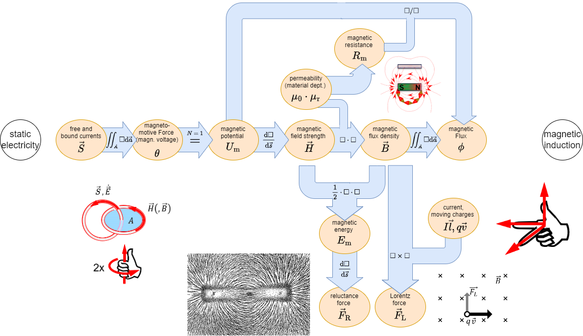
In the previous chapters we got accustomed to the magnetic field. During this path some similarities from the magnetic field to the electric circuit appeared (see Abbildung 1).

In this chapter we will investigate, how far we come with such an analogy and where it can by practically applied.
5.1 Linear magnetic Circuits
For the upcoming calculations the following assumptions are made
- The relationship between $B$ and $H$ is linear: $B = \mu \cdot H$
This is a good estimation when the magnetic field strength lays well below saturation - There is not stray field leaking out of the magnetic-field conducting material.
- The fields inside of airgaps is homogenious. This is true for small airgaps.
One can calulate a lot of simple magnetic circuits, when this assumptions and focusing on the average field line are applied.

Two simple magnetic circuits are shown in Abbildung 3: They consist of
- a current-carrying coil
- a ferrite core
- an airgap (in picture (2) ).

This three parts will be investigated shortly:
Current-carrying Coil
For the magnetic circuit, the coil is parameterized only by:
- its nuber of windings $N$ and
- the passing current $i$.
This parameters lead to the magnetic voltage $\theta = N\cdot i$.
Ferrite Core
- The core is assumed to be made of ferromagnetic material.
- Therefore, the relative permeability in the core is much larger than in air ($\mu_{r,core}>>1$).
- The ferrite core is also filling the inside of the current-carrying coil.
- The ferrite core conducts the magnetic flux around the magnetic circuit (and by this: also to the airgap)
Airgap
- The airgap interrupts the ferrite core.
- The width of the airgap is small compared to the dimensions of the cross section of the ferrite core.
- The field in the airgap can be used to generate (mechanical) effects within the airgap.
An example for this can be the force onto a permanent magnet (see Abbildung 3 (3)).
With the above-mentioned assumtions the magnetic flux $\Phi$ must remain constant along the ferrite core, so $\Phi_{core}=const.$.
Since the magnetic field lines to neither show sources nor sinks, also the flux passing over to the airgap must be $\Phi_{airgap}=\Phi_{core}=const.$
This can also be seen in Abbildung 4 (1) ).
A different view onto this is the closed surface $\vec{A}$ (Abbildung 4 (2)): Based on the examination in Recap of magnetic Field we know that the flux into the volume must be equal the flux out of the volume, or $\Phi_m = \iint_{A} \vec{B} \cdot d \vec{A} = 0$.
The relationship $B=\mu \cdot H$, and $\mu_{core}\gg\mu_{airgap}$ lead to the fact that the ${H}$-Field must be much stronger within the airgap (Abbildung 4 (3)).

Magnetic Cirtuit in a Formula
Therefore, the following formula is given \begin{align*} \Phi_m &= &\iint_A &\vec{B} \cdot d \vec{A} &= &const. \\ &= & &B \cdot A &= &const. \\ &= & &B_{core} \cdot A_{core} &= &B_{airgap} \cdot A_{airgap} = const. \\ \end{align*}
The assumptions, that there is that the field inside of airgap is homogenious and there is no strayfield lead to the fact, that $A_{core} = A_{airgap}$.
Therefore:
\begin{align*}
B_{core} &= &B_{airgap} = B \\
\mu_0 \mu_{r,core} H_{core} &= &\mu_0 \mu_{r,airgap} H_{airgap} = {{\Phi}\over{A}} \tag{5.2.1}
\end{align*}
Beside this, the magnetic field strength $H$ along one field line is directly given by: \begin{align*} \theta = N \cdot i &= \int_s \vec{H} d\vec{s} = \\ &= \int_{core} \vec{H} d\vec{s} + \int_{airgap} \vec{H} d\vec{s} \\ \end{align*}
With the assumtion of a linear and homogeneous $B$-Field and the width $\delta$ of the airgap, this leads to: \begin{align*} \theta = {H}_{core} l_{core} + {H}_{airgap} \delta \tag{5.2.2} \end{align*}
With the prevoius formula $5.2.1$, this gets to: \begin{align*} \theta &= {{B}\over{\mu_0 \mu_{r,core}}} l_{core} + {{B}\over{\mu_0 \mu_{r,airgap}}} \delta \\ &= {{\Phi \cdot l_{core}}\over{A \cdot \mu_0 \mu_{r,core}}} + {{\Phi \cdot \delta}\over{A \cdot \mu_0 \mu_{r,airgap}}} \\ &= {{1}\over{\mu_0 \mu_{r,core}}}{{l_{core}}\over{A}} \cdot \Phi + {{1}\over{\mu_0 \mu_{r,airgap}}}{{\delta}\over{A}} \cdot \Phi \tag{5.2.3} \end{align*}
Comparing the formula $5.2.3$ with the ohmic resistance and resistivity of two resistors in series, shows something interesting: \begin{align*} u &= &R_1 \cdot &i &+ &R_2 \cdot i \\ &= &\rho {{l_1}\over{A_1}} \cdot &i &+ &\rho {{l_2}\over{A_2}} \cdot i \end{align*}
This leads to:
- The magnetic voltage $\theta$ acts like the electic voltage $u$,
the magnetic flux $\Phi$ like the current $i$. - The linear relationship $\theta = f(\Phi)$ is also called Hopkinson's Law.
Notice:
- Also for the magnetic circuit one can set up a lumped circuit model (see Abbildung 5).
- Similar to Ohms law, there is a magnetic resistance or reluctance:
\begin{align*} \boxed{R_m = {{1}\over{\mu_0 \mu_{r}}}{{l}\over{A}}} \end{align*} - The unit of $R_m$ is $[R_m]= [\theta]/[\Phi] = 1 A / Vs = 1/H $
- The length $l$ is given by the average field line length in the core.
- The Kirchhoff's laws (mesh rule and nodal rule) can also be applied:
- The sum of the magentic fluxes $\Phi_i$ in into a node is: $\sum_i \Phi_i=0 $
- The sum of the magnetic voltages $\theta_i$ along the average field line is: $\sum_i \theta_i=0 $
- The application of the lumped circuit model is based on multiple assumptions.
In contrast to the simplification for the electric current and voltage the simplification for the flux and magnetic voltage in not as exact.

Application and Limitations of the Circuit Interpretation
Notice:
„Recipe“ for solving magnetic circuits:- Watch out for indicidual magnetic resistances in the circuits:
- Separate the magnetic circuit into parts, where the the permeability and area of the cross section is constant.
For these parts $B$ and $H$ is constant. These parts will have individual magnetic resistances. - Each airgap also gest an individual magnetic resistance.
- Calculate the magnetic resistance by the average length of field line through the individual parts.
- Calculate the magnetic circuit as circuit.
- Magnetic voltages depicts voltage sources ; magnetic flux depicts currents.
- Use the known way to solve the circuit.
Be aware that the orientation of the current $I$ and the field strength $\vec{H}$ are also connected by the right hant rule.
The results are only allowed as first approximation. The following table shows the contrast between the electric and magnetic field:
| Property | Electric Field | Magnetic Field |
|---|---|---|
| Materials | There are „pure“ isolator, which are completely non conductive. | All materials have a permeability $>0$ |
| Sources | The source is concentrated (= there are field sources / electric charges) | The magnetic source (= coil) is distributed |
| Simplifications | The simplifications often work for good results (small wire diameter, relativly constant resistivity) | The simplification are often too simple (wide spread beyond the average field length, non-linearity of the permeability) |
Task 5.1.1 Coil on a plastic Core
A coil is set-up onto a toroidal plastic ring ($\mu_r=1$) with an average circumference of $l_R = 300mm$. The $N=400$ windings are evenly distributed along the circumference. The diameter on the cross section of the plastic ring is $d = 10mm$. In the windings a current of $I=500mA$ is flowing.
Calculate
- the magnetic field strength $H$ in the middle of the ring cross section.
- the magnetic flux density $B$ in the middle of the ring cross section.
- the magnetic resistance $R_m$ of the plastic ring.
- the magnetic flux $\Phi$.
Task 5.1.2 Coil on a ferrite Core with airgap
The choke coil shown in Abbildung 10 shall be given, with a constant cross section in all legs $l_0$, $l_1$, $l_2$. The number of windings shall be $N$ and the current through a single winding $I$.

- Draw the lumped circuit of the magnetic system
- Calculate all magnetic resistances $R_{m,i}$
- Calculate the partial fluxes in al the legs of the circuit
5.2 Non-linear magnetic Circuits
not included in the present script
5.3 Mutual Induction and Coupling
Situation: Two coils $1$ and $2$ near by each other.
Which effect do the coils have onto each other?

Effect of Coils onto each other
- Windings $N_1$ of coil $1$ gets feed with current $i_1$.
- Coil $1$ generates change in flux $\Phi_{11}$
- Coil $2$ gets passed by part of the flux ($\Phi_{21}$)
- Stray flux $\Phi_{S1}$ takes not part in coupling
- $\rightarrow$ Coils are magnetically coupled:
Flux $\Phi_{11}$ of coil $1$ gets divided into flux $\Phi_{21}$ in coil $2$ and stray flux $\Phi_{S1}$ not passing coil $2$:
$\Phi_{11} = \Phi_{21} + \Phi_{S1}$
- Induced voltage in coil $2$:
$ u_{ind,2} = -{{d}\over{dt}}\Psi_{21} $
$\quad\quad = -N_2 \cdot {{d}\over{dt}}\Phi_{21} $
- Similar effect on coil $1$ due to a current $i_2$ through coil $2$:
$\Phi_{22} = \Phi_{12} + \Phi_{S2}$
$ u_{ind,1} = -N_1 \cdot {{d}\over{dt}}\Phi_{12} $
Linked Fluxes
For the single coil we got the relationship between the linked flux $\Psi$ and the current $i$ as: $\Psi = L \cdot i$.
Now the coils also are interacting with each other. This must also be reflected in the relationship $\Psi_1 = f(i_1, i_2)$, $\Psi_2 = f(i_1, i_2)$:
\begin{align*}
\Psi_1 &= &L_{11} &\cdot i_1 &+ M_{12} &\cdot i_2 \\
\Psi_2 &= &L_{22} &\cdot i_2 &+ M_{21} &\cdot i_1 \\
\end{align*}
With
- $L_{11}$ and $L_{22}$ as the self induction
- $M_{12}$ and $M_{21}$ as the mutual induction
The formula can also be described as: \begin{align*} \left( \begin{array}{c} \Psi_1 \\ \Psi_2 \end{array} \right) = \left( \begin{array}{c} L_{11} & M_{12} \\ M_{21} & L_{22} \end{array} \right) \cdot \left( \begin{array}{c} i_1 \\ i_2 \end{array} \right) \end{align*}
The main question is now: How do we get $L_{11}$, $M_{12}$, $L_{22}$, $M_{21}$?
Magnetic Circuit with 2 Sources
In order to get the self induction and mutual induction of two interacting coils, we are going to investigate two coils on an iron core with a middle leg (see Abbildung 10).
Ther the stray flux of the previous situation is only located in the middle leg.
This also means, that there is no stray flux outside of the iron core.

The Abbildung 10 shows the fluxes on each parts. The filled black circles nearby the windings mark the direction of winding:
When there is one current for each winding ingoing into the marked pin, the fluxes will get added up positively.
In order to get $L_{11}$ and $L_{22}$, we look back to the inductivity $L$ of a long coil with the length $l$.
This was given in the chapter Self-Induction as
\begin{align*} L &= {{\Psi}\over{i}} \\ L &= \mu_0 \mu_r \cdot N^2 \cdot {{A }\over {l}} \\ \end{align*}
In this case, $\Psi$ was the flux through the coil generated from the coil itself - here $L_{11}$ and $L_{22}$.
Comparing this formula with the magnetic resistance $R_m = {{1}\over{\mu_0 \mu_{r}}}{{l}\over{A}}$ of the coil, one can conclude:
\begin{align} \boxed{L = {{N^2 }\over {R_{m,coil}}}} \end{align}
Based on this formula, the self inductions $L_{11}$ and $L_{22}$ can be written with the magnetic resistances of the coils as:
\begin{align*} L_{11} &= {{N_1^2 }\over {R_{m,11}}} \\ L_{22} &= {{N_2^2 }\over {R_{m,22}}} \end{align*}
In order to get the effect of the mutual induction, a coupling coefficient $k$ is introduced. $k_{21}$ describes how much of the flux from coil $1$ is acting on coil $2$ (similar for $k_{12}$):
\begin{align*} k_{21} = {{\Phi_{21}}\over{\Phi_{11}}} \\ \end{align*}
When $k_{21}=100\%$, there is no flux in the middle leg but only in the second coil.
For $k_{21}=0\%$ all the flux is in the middle leg circumventing the second coil, i.e. there is no coupling.
The resulting total coupling $k$ is given as
\begin{align*} k = \sqrt{k_{12}\cdot k_{21}} \\ \end{align*}
The mutual induction $M_{21}$ can be calculated as the fraction of the linked flux $\Psi_{11}$ from coil $1$ acting on the current $i_2$ of coil $2$:
\begin{align*} M_{21} &= {{\Psi_{21}}\over{i_2}} \\ &= {{N_2 \cdot \Phi_{21}}\over{i_2}} \\ &= {{N_2 \cdot k_{21} \cdot \Phi_{11}}\over{i_2}} \\ &= {{N_2}\over{N_1}}k_{21} \cdot {{\Psi_{11}}\over{i_2}} \\ &= {{N_2}\over{N_1}}k_{21} \cdot L_{11} \\ &= {{N_2}\over{N_1}}k_{21} \cdot {{N_1^2 }\over {R_{m,11}}} \\ &= k_{21} \cdot {{N_1 \cdot N_2 }\over {R_{m,11}}} \\ \end{align*}
\begin{align*} M_{21} &= {{\Psi_{21}}\over{i_2}} \\ &= {k_{21} \cdot {\Psi_{11}}\over{i_2}} \\ &= {k_{21} \cdot N_1 \cdot {\Phi_{11}}\over{i_2}} \\ \end{align*}
\begin{align*} L \cdot i = \Psi_{11} &= N_1 \cdot \Phi_{11} \\ \end{align*}
With the
The formula can also be described as: \begin{align*} \left( \begin{array}{c} \Psi_1 \\ \Psi_2 \end{array} \right) = \left( \begin{array}{c} L_{11} & M_{12} \\ M_{21} & L_{22} \end{array} \right) \cdot \left( \begin{array}{c} i_1 \\ i_2 \end{array} \right) \end{align*}
5.4 Magnetic Energy
Tasks
Task 5.1.4 Application: Shaded Pole Motor
The Abbildung 22 and Abbildung 22 show a shaded pole motor of a commercial oven.
- Find out how this motor works - explicitly: why is there a prefered direction of the motor?
- In which direction does the shown motor run?