This is an old revision of the document!
5. Magnetic Circuits
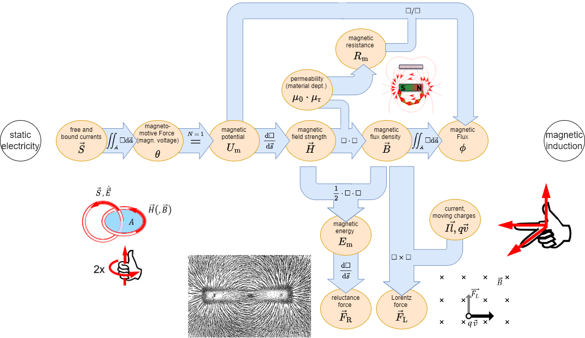
In the previous chapters we got accustomed tof the magnetic field. During this path some similarities from the magnetic field to the electric circuit appeared (see figure 1).

In this chapter we will investigate, how far we come with such an analogy and where it can by practically applied.
5.1 Linear magnetic Circuits
For the upcoming calculations the following assumptions are made
- The relationship between $B$ and $H$ is linear: $B = \mu \cdot H$
This is a good estimation when the magnetic field strength lays well below saturation - There is not stray field leaking out of the magnetic-field conducting material.
- The fields inside of airgaps is homogenious. This is true for small airgaps.
One can calulate a lot of simple magnetic circuits, when this assumptions and focusing on the average field line are applied.

Two simple magnetic circuits are shown in figure 3: They consist of
- a current-carrying coil
- a ferrite core
- an airgap (in picture (2) ).

This three parts will be investigated shortly:
Current-carrying Coil
For the magnetic circuit, the coil is parameterized only by:
- its nuber of windings $N$ and
- the passing current $i$.
This parameters lead to the magnetic voltage $\theta = N\cdot i$.
Ferrite Core
- The core is assumed to be made of ferromagnetic material.
- Therefore, the relative permeability in the core is much larger than in air ($\mu_{r,core}\gg 1$).
- The ferrite core is also filling the inside of the current-carrying coil.
- The ferrite core conducts the magnetic flux around the magnetic circuit (and by this: also to the airgap)
Airgap
- The airgap interrupts the ferrite core.
- The width of the airgap is small compared to the dimensions of the cross section of the ferrite core.
- The field in the airgap can be used to generate (mechanical) effects within the airgap.
An example for this can be the force onto a permanent magnet (see figure 3 (3)).
With the above-mentioned assumtions the magnetic flux $\Phi$ must remain constant along the ferrite core, so $\Phi_{core}=const.$.
Since the magnetic field lines to neither show sources nor sinks, also the flux passing over to the airgap must be $\Phi_{airgap}=\Phi_{core}=const.$
This can also be seen in figure 4 (1) ).
A different view onto this is the closed surface $\vec{A}$ (figure 4 (2)): Based on the examination in Recap of magnetic Field we know that the flux into the volume must be equal the flux out of the volume, or $\Phi_m = \iint_{A} \vec{B} \cdot d \vec{A} = 0$.
The relationship $B=\mu \cdot H$, and $\mu_{core}\gg\mu_{airgap}$ lead to the fact that the ${H}$-Field must be much stronger within the airgap (figure 4 (3)).

Magnetic Circuit in a Formula
Therefore, the following formula is given \begin{align*} \Phi_m &= &\iint_A &\vec{B} \cdot d \vec{A} &= &const. \\ &= & &B \cdot A &= &const. \\ &= & &B_{core} \cdot A_{core} &= &B_{airgap} \cdot A_{airgap} = const. \\ \end{align*}
The assumptions, that there is that the field inside of airgap is homogenious and there is no strayfield lead to the fact, that $A_{core} = A_{airgap}$.
Therefore:
\begin{align*}
B_{core} &= &B_{airgap} = B \\
\mu_0 \mu_{r,core} H_{core} &= &\mu_0 \mu_{r,airgap} H_{airgap} = {{\Phi}\over{A}} \tag{5.2.1}
\end{align*}
Beside this, the magnetic field strength $H$ along one field line is directly given by: \begin{align*} \theta = N \cdot i &= \int_s \vec{H} d\vec{s} = \\ &= \int_{core} \vec{H} d\vec{s} + \int_{airgap} \vec{H} d\vec{s} \\ \end{align*}
With the assumtion of a linear and homogeneous $B$-Field and the width $\delta$ of the airgap, this leads to: \begin{align*} \theta = {H}_{core} l_{core} + {H}_{airgap} \delta \tag{5.2.2} \end{align*}
With the prevoius formula $5.2.1$, this gets to: \begin{align*} \theta &= {{B}\over{\mu_0 \mu_{r,core}}} l_{core} + {{B}\over{\mu_0 \mu_{r,airgap}}} \delta \\ &= {{\Phi \cdot l_{core}}\over{A \cdot \mu_0 \mu_{r,core}}} + {{\Phi \cdot \delta}\over{A \cdot \mu_0 \mu_{r,airgap}}} \\ &= {{1}\over{\mu_0 \mu_{r,core}}}{{l_{core}}\over{A}} \cdot \Phi + {{1}\over{\mu_0 \mu_{r,airgap}}}{{\delta}\over{A}} \cdot \Phi \tag{5.2.3} \end{align*}
Comparing the formula $5.2.3$ with the ohmic resistance and resistivity of two resistors in series, shows something interesting: \begin{align*} u &= &R_1 \cdot &i &+ &R_2 \cdot i \\ &= &\rho {{l_1}\over{A_1}} \cdot &i &+ &\rho {{l_2}\over{A_2}} \cdot i \end{align*}
This leads to:
- The magnetic voltage $\theta$ acts like the electic voltage $u$,
the magnetic flux $\Phi$ like the current $i$. - The linear relationship $\theta = f(\Phi)$ is also called Hopkinson's Law.
Notice:
- Also for the magnetic circuit one can set up a lumped circuit model (see figure 5).
- Similar to Ohms law, there is a magnetic resistance or reluctance:
\begin{align*} \boxed{R_m = {{1}\over{\mu_0 \mu_{r}}}{{l}\over{A}}} \end{align*} - The unit of $R_m$ is $[R_m]= [\theta]/[\Phi] = 1 A / Vs = 1/H $
- The length $l$ is given by the average field line length in the core.
- The Kirchhoff's laws (mesh rule and nodal rule) can also be applied:
- The sum of the magentic fluxes $\Phi_i$ in into a node is: $\sum_i \Phi_i=0 $
- The sum of the magnetic voltages $\theta_i$ along the average field line is: $\sum_i \theta_i=0 $
- The application of the lumped circuit model is based on multiple assumptions.
In contrast to the simplification for the electric current and voltage the simplification for the flux and magnetic voltage in not as exact.

Application and Limitations of the Circuit Interpretation
Notice:
“Recipe” for solving magnetic circuits:- Watch out for indicidual magnetic resistances in the circuits:
- Separate the magnetic circuit into parts, where the the permeability and area of the cross section is constant.
For these parts $B$ and $H$ is constant. These parts will have individual magnetic resistances. - Each airgap also gest an individual magnetic resistance.
- Calculate the magnetic resistance by the average length of field line through the individual parts.
- Calculate the magnetic circuit as circuit.
- Magnetic voltages depicts voltage sources ; magnetic flux depicts currents.
- Use the known way to solve the circuit.
Be aware that the orientation of the current $I$ and the field strength $\vec{H}$ are also connected by the right hant rule.
The results are only allowed as first approximation. The following table shows the contrast between the electric and magnetic field:
| Property | Electric Field | Magnetic Field |
|---|---|---|
| Materials | There are “pure” isolator, which are completely non conductive. | All materials have a permeability $>0$ |
| Sources | The source is concentrated (= there are field sources / electric charges) | The magnetic source (= coil) is distributed |
| Simplifications | The simplifications often work for good results (small wire diameter, relativly constant resistivity) | The simplification are often too simple (wide spread beyond the average field length, non-linearity of the permeability) |
Task 5.1.1 Coil on a plastic Core
A coil is set-up onto a toroidal plastic ring ($\mu_r=1$) with an average circumference of $l_R = 300mm$. The $N=400$ windings are evenly distributed along the circumference. The diameter on the cross section of the plastic ring is $d = 10mm$. In the windings a current of $I=500mA$ is flowing.
Calculate
- the magnetic field strength $H$ in the middle of the ring cross section.
- the magnetic flux density $B$ in the middle of the ring cross section.
- the magnetic resistance $R_m$ of the plastic ring.
- the magnetic flux $\Phi$.
Task 5.1.2 Coil on a ferrite Core with airgap
The choke coil shown in figure 10 shall be given, with a constant cross section in all legs $l_0$, $l_1$, $l_2$. The number of windings shall be $N$ and the current through a single winding $I$.

- Draw the lumped circuit of the magnetic system
- Calculate all magnetic resistances $R_{m,i}$
- Calculate the partial fluxes in al the legs of the circuit
5.2 Non-linear magnetic Circuits
not included in the present script
5.3 Mutual Induction and Coupling
Situation: Two coils $1$ and $2$ near by each other.
Questions:
- Which effect do the coils have onto each other?
- Can we describe the effects with mainly electric properties (i.e. no gemoetric properties)

Effect of Coils onto each other
- Windings $N_1$ of coil $1$ gets feed with current $i_1$.
- Coil $1$ generates change in flux $\Phi_{11}$
- Coil $2$ gets passed by part of the flux ($\Phi_{21}$)
- Stray flux $\Phi_{S1}$ takes not part in coupling
- $\rightarrow$ Coils are magnetically coupled:
Flux $\Phi_{11}$ of coil $1$ gets divided into flux $\Phi_{21}$ in coil $2$ and stray flux $\Phi_{S1}$ not passing coil $2$:
$\Phi_{11} = \Phi_{21} + \Phi_{S1}$
- Induced voltage in coil $2$:
$ u_{ind,2} = -{{d}\over{dt}}\Psi_{21} $
$\quad\quad = -N_2 \cdot {{d}\over{dt}}\Phi_{21} $
- Similar effect on coil $1$ due to a current $i_2$ through coil $2$:
$\Phi_{22} = \Phi_{12} + \Phi_{S2}$
$ u_{ind,1} = -N_1 \cdot {{d}\over{dt}}\Phi_{12} $
Linked Fluxes
For the single coil we got the relationship between the linked flux $\Psi$ and the current $i$ as: $\Psi = L \cdot i$.
Now the coils also are interacting with each other. This must also be reflected in the relationship $\Psi_1 = f(i_1, i_2)$, $\Psi_2 = f(i_1, i_2)$:
\begin{align*}
\Psi_1 &= &\Psi_{11} &+ \Psi_{12} \\
\Psi_2 &= &\Psi_{22} &+ \Psi_{21} \\
\\
\Psi_1 &= &L_{11} \cdot i_1 &+ M_{12} \cdot i_2 \\
\Psi_2 &= &L_{22} \cdot i_2 &+ M_{21} \cdot i_1 \\
\end{align*}
With
- $L_{11}$ and $L_{22}$ as the self induction
- $M_{12}$ and $M_{21}$ as the mutual induction
The formula can also be described as: \begin{align*} \left( \begin{array}{c} \Psi_1 \\ \Psi_2 \end{array} \right) = \left( \begin{array}{c} L_{11} & M_{12} \\ M_{21} & L_{22} \end{array} \right) \cdot \left( \begin{array}{c} i_1 \\ i_2 \end{array} \right) \end{align*}
The view onto the magnetic flux is sometimes good, when effects like an acting Lorentz force in at interest. More often the coils are coupling two electric circuits linke in a transformer or a wireless charger. Here, the effect into the circuits is of interest. This can be calculated with the induced electric voltages $u_{ind,1}$ and $u_{ind,2}$ in each circuits. They are given by the formula $u_{ind,x} = -d\Psi_x /dt$:
\begin{align*} \left( \begin{array}{c} u_1 \\ u_2 \end{array} \right) &= -{{d}\over{dt}} \left( \begin{array}{c} \Psi_1 \\ \Psi_2 \end{array} \right) \\ &= -\left( \begin{array}{c} L_{11} & M_{12} \\ M_{21} & L_{22} \end{array} \right) \cdot \left( \begin{array}{c} {{d}\over{dt}}i_1 \\ {{d}\over{dt}}i_2 \end{array} \right) \end{align*}
The main question is now: How do we get $L_{11}$, $M_{12}$, $L_{22}$, $M_{21}$?
Magnetic Circuit with 2 Sources
In order to get the self induction and mutual induction of two interacting coils, we are going to investigate two coils on an iron core with a middle leg (see figure 10).
Ther the stray flux of the previous situation is only located in the middle leg.
This also means, that there is no stray flux outside of the iron core.

The figure 10 shows the fluxes on each parts. The black dots nearby the windings mark the direction of winding:
When there is one current for each winding ingoing into the marked pin, the fluxes will get added up positively.
In order to get $L_{11}$ and $L_{22}$, we look back to the inductivity $L$ of a long coil with the length $l$.
This was given in the chapter Self-Induction as
\begin{align*} L &= {{\Psi}\over{i}} \\ L &= \mu_0 \mu_r \cdot N^2 \cdot {{A }\over {l}} \\ \end{align*}
In this case, $\Psi$ was the flux through the coil generated from the coil itself - here $L_{11}$ and $L_{22}$.
Comparing this formula with the magnetic resistance $R_m = {{1}\over{\mu_0 \mu_{r}}}{{l}\over{A}}$ of the coil, one can conclude:
\begin{align} L = {{N^2 }\over {R_{m,coil}}} \end{align}
Important here is, that we assumed no stray field. When taking this into account for calculating the self induction the magnetic resistance $R_{m,coil}$ ends op to be the resistance of the magnetic circuit, seen by the magnetic voltage source!
\begin{align} \boxed{L = {{N^2 }\over {R_{m1}}}} \end{align}
The magnetic resistance $R_{m1}$ in the example figure 10 is $R_{m1} = R_{m,11} + (R_{m,ss}||R_{m,22})$. Based on this formula, the self inductions $L_{11}$ and $L_{22}$ can be written with the magnetic resistances of the coils as:
\begin{align*} L_{11} &= {{N_1^2 }\over {R_{m1}}} \\ L_{22} &= {{N_2^2 }\over {R_{m2}}} \end{align*}
In order to get the effect of the mutual induction, a coupling coefficient $k$ is introduced. $k_{21}$ describes how much of the flux from coil $1$ is acting on coil $2$ (similar for $k_{12}$):
\begin{align*} k_{21} = {{\Phi_{21}}\over{\Phi_{11}}} \\ \end{align*}
When $k_{21}=100\%$, there is no flux in the middle leg but only in the second coil.
For $k_{21}=0\%$ all the flux is in the middle leg circumventing the second coil, i.e. there is no coupling.
The mutual induction $M_{21}$ can be calculated as the fraction of the linked flux $\Psi_{11}$ in coil $2$ based on the current $i_1$ from the coil $1$ :
\begin{align*} M_{21} &= {{\Psi_{21}}\over{i_1}} \\ &= {{N_2 \cdot \Phi_{21}}\over{i_1}} \\ &= {{N_2 \cdot k_{21} \cdot \Phi_{11}}\over{i_1}} \\ &= {{N_2}\over{N_1}}k_{21} \cdot {{\Psi_{11}}\over{i_1}} \\ &= {{N_2}\over{N_1}}k_{21} \cdot L_{11} \\ &= {{N_2}\over{N_1}}k_{21} \cdot {{N_1^2 }\over {R_{m1}}} \\ &= k_{21} \cdot {{N_1 \cdot N_2 }\over {R_{m1}}} \\ \end{align*}
The formula is finally: \begin{align*} \left( \begin{array}{c} \Psi_1 \\ \Psi_2 \end{array} \right) = \left( \begin{array}{c} {{N_1^2}\over{R_{m1}}} & k_{12}\cdot{{N_1 \cdot N_2}\over{R_{m2}}} \\ k_{21}\cdot{{N_1 \cdot N_2}\over{R_{m1}}} & {{N_2^2}\over{R_{m2}}} \end{array} \right) \cdot \left( \begin{array}{c} i_1 \\ i_2 \end{array} \right) \end{align*}
Task 5.3.1 Example for magnetic Circuit with two Sources
The magnetical configuration in figure 11 shall be given.
The area of the cross-section is $A=9cm^2$ in all parts, the permeability is $\mu_r=800$, the length $l=12cm$ and the number of windings $N_1 = 400$, $N_2=300$. The coupling factors are $k_{12}=0.6$ and $k_{21}=0.8$.
Calculate $L_{11}$, $M_{12}$, $L_{22}$, $M_{21}$.

Step 1: Draw the problem as a network
Step 2: Calculate the magnetic resistances
The magnetic resistance is summed up looking at the circuit from the source $1$: \begin{align*} R_{m1} &= R_{m,11} + R_{m,ss} || R_{m,22} \\ \end{align*}
where the parts are given as \begin{align*} R_{m,11} &= {{1}\over{\mu_0 \mu_{r}}}{{3\cdot l}\over{A}} \\ R_{m,ss} &= {{1}\over{\mu_0 \mu_{r}}}{{1\cdot l}\over{A}} \\ R_{m,22} &= {{1}\over{\mu_0 \mu_{r}}}{{2\cdot l}\over{A}} \\ \end{align*}
With the given geometry this leads to \begin{align*} R_{m1} &= {{1}\over{\mu_0 \mu_{r}}}{{l}\over{A}}\cdot (3 + {{1\cdot 2}\over{1 + 2}}) \\ &= {{1}\over{\mu_0 \mu_{r}}}{{l}\over{A}}\cdot {{11}\over{3}} \\ &= 133 \cdot 10^{3} \cdot {{11}\over{3}} {{1}\over{H}}\\ \end{align*}
Similarly, the magnetic resistance $R_{m2}$ is \begin{align*} R_{m2} &= {{1}\over{\mu_0 \mu_{r}}}{{l}\over{A}}\cdot {{11}\over{4}} \\ &= 133 \cdot 10^{3} \cdot {{11}\over{4}} {{1}\over{H}}\\ \end{align*}
Step 3: Calculate the magnetic inductances
\begin{align*} L_{11} &= {{N_1^2}\over{R_{m1}}} &= 329 mH\\ \\ L_{22} &= {{N_2^2}\over{R_{m2}}} &= 247 mH\\ \\ M_{21} &= k_{21}\cdot{{N_1 \cdot N_2}\over{R_{m1}}} &= 197 mH\\ \\ M_{12} &= k_{12}\cdot{{N_1 \cdot N_2}\over{R_{m2}}} &= 197 mH\\ \end{align*}
For symmetrical magnetic structures and $\mu_r = const.$ the following applies:
- the mutual inductances are equal: $M_{12}=M_{21}=M$
- the mutual inductance $M$ is: $M = \sqrt{M_{12}\cdot M_{21}} = k \cdot \sqrt {L_{11}\cdot L_{22}}$
- The resulting *total coupling* $k$ is given as \begin{align*} k = \sqrt{k_{12}\cdot k_{21}} \end{align*}
Effects in the electic circuits
- Whenever two coils are magnetically coupled, not only the self induction $L$, but also the mutual induction $M$ applies.
- Based on the currents $i_1$, $i_2$ in the two circuits, the induced voltages are given by:
\begin{align*} u_1 &= L_{11} \cdot {{di_1}\over{dt}} &+ M \cdot {{di_2}\over{dt}} & \\ u_2 &= M \cdot {{di_1}\over{dt}} &+ L_{22} \cdot {{di_2}\over{dt}} & \\ \end{align*}
It is important to consider the polarity of the fluxes for the calculation in circuits (see figure 15). The sign of the mudual induction is influenced by
- the direction of the windings
- the orientation / counting of the current in the circuit

positive Polarity
The polarity is positive, when both currents either flowing into or out of the dotted pin (see figure 16).
Fig. 16: Example Circuits with positive Polarity

In this case the mutual induction added positivly.
The formula of the shown circuitry is then: \begin{align*} u_1 &= R_1 \cdot i_1 &+ L_{11} \cdot {{di_1}\over{dt}} &+ M \cdot {{di_2}\over{dt}} & \\ u_2 &= R_2 \cdot i_2 &+ L_{22} \cdot {{di_2}\over{dt}} &+ M \cdot {{di_1}\over{dt}} & \\ \end{align*}
negative Polarity
The polarity is negative, when only one current either flows into the dotted pin and the other one out of the dotted pin (see figure 17).

In this case the mutual induction added negativly.
The formula of the shown circuitry is then: \begin{align*} u_1 &= R_1 \cdot i_1 &+ L_{11} \cdot {{di_1}\over{dt}} &- M \cdot {{di_2}\over{dt}} & \\ u_2 &= R_2 \cdot i_2 &+ L_{22} \cdot {{di_2}\over{dt}} &- M \cdot {{di_1}\over{dt}} & \\ \end{align*}
5.4 Magnetic Energy
The magnetic field of a coil stores magnetic energy. The energy transfer from the electric circuit to the magentic field is also the cause for the “current dampening” effect of the inductor. The energetic turnover for charging an conductor from $i(t_0=0)=0$ to $i(t_1)=I$ is given by:
\begin{align*} W_m = \int_0^\infty u(t)\cdot i(t) dt \end{align*}
With $u_L = L \cdot di/dt$, this becomes:
\begin{align*} W_m &= \int_0^\infty L\cdot {{di}\over{dt}}\cdot i(t) dt \\ &= \int_0^\infty L\cdot i(t) di \\ &= L\cdot \int_0^\infty i(t) di \\ &= L\cdot \left[ {{1}\over{2}}i^2\right]_0^I \\ \boxed{W_m = {{1}\over{2}}L\cdot I^2 } \end{align*}
magnetic Energy of a magnetic Circuit
With this formula also the stored energy in a macnetic circuit can be calculated. For this, the formula be rewritten by the properties linked flux $\Psi = N\cdot \Phi = L\cdot I$ and magnetic voltage $\theta=N\cdot I = \Phi \cdot R_m$ of the magnetic circuit: \begin{align*} \boxed{W_m = {{1}\over{2}}\Psi\cdot I = {{1}\over{2}}{{\Psi^2 }\over{L}}} \end{align*}
magnetic Energy of a toroid Coil
The formula can also be used for caclulating the stored energiy of a toroid coil with $N$ windings, the cross section $A$ and an average length $l$ of a field line. By ths, the following formulas can be used: \begin{align*} \theta = H\cdot l = N\cdot I \\ \Phi = B \cdot A \end{align*}
With the above-mentioned formulas of the magnetic circuit we get: \begin{align*} W_m &= {{1}\over{2}}\Psi\cdot I \\ &= {{1}\over{2}}N\cdot B \cdot A \cdot {{H\cdot l}\over{N}} \\ &= {{1}\over{2}}B \cdot H \cdot A \cdot l \\ \end{align*} \begin{align*} \boxed{W_m = {{1}\over{2}}B\cdot H \cdot V} \end{align*}
The magnetic energy density $w_m$ can therefore be calculated as: \begin{align*} w_m &= {{W_m}\over{V}} \\ &= {{1}\over{2}}B \cdot H \\ \end{align*}
This formula is also true for other types of coils.
generalized magnetic Energy
The general term to find the magnetic energy (e.g. for inhomogenious magnetic fields) is given by \begin{align*} W_m &= \iiint_V{w_m dV} \\ &= \iiint_V{\vec{B}\cdot \vec{H} dV} \end{align*}
Application of the magnetic Energy
The circuit shown in figure 21 shall now be investigated. The inductor shall be a toroid coil with $N$ windings, the cross section $A$ and an average length $l$ of a field line.

The Kirchhoff mesh law leads to:
\begin{align*} u_s = u_R + u_L \\ u_s = R \cdot i + N {{d\Phi}\over{dt}} \end{align*}
Multipling with $i$ and with $dt$ we get the principle of conservation of energy $dw = u \cdot i \cdot dt$ for each small time step.
\begin{align*} u_s \cdot i \cdot dt &= R \cdot i^2 \cdot dt &+ N {{d\Phi}\over{dt}} \cdot i \cdot dt & \\ dW &= dW_R &+ dW_m \end{align*}
On this way we get the magnetic energy as: \begin{align*} dW_m &= N {{d\Phi}\over{dt}} \cdot i \cdot dt \\ W_m &= \int dW_m \\ &= N \int_0^t {{d\Phi}\over{dt}} \cdot i \cdot dt \\ &= N \int_0^{\Phi} i \cdot d\Phi \\ \end{align*}
In a toriod coil with a given cross section $A$ the flux change $d\Phi$ can only be given as a change in the field $B$. Therefore, $d\Phi = A \cdot dB$. Additionally, we know that the magnetic voltage is given by $\theta(t) = N \cdot i = H(t) \cdot l$. Inluding this into the formula gives us:
\begin{align*} W_m &= N \int_0^{B} i \cdot A \cdot dB \\ &= \int_0^{B} H(B) \cdot l\cdot A \cdot dB \\ &= V\int_0^{B} H(B) \cdot dB \\ \end{align*}
We can conclude that the magnetic energy $W_m$: $W_m$ can be calculated from the $H$-$B$-curve by integrating the external magnetic field strength $H$ for each small step of the flux density $dB$. This wil be shown for the case of a linear magnetic behavior, a nonlinear behavior and the situation with magentic hysteresis shortly.
Circuit with linear magnetic Behavior
In figure 22 the situation for a magnetic material with a linear relationship between $B$ and $H$ is shown. Given by the maximum current $I_{max}$ the maximum field strength $H_{max}$ can be derived. In the circuit in figure 21, the inductor will experience increasing and decreasing current. Therefore, the $B$-$H$-curve gets passed through positive and negative values of $H$ and $H$ along the line of $B=\mu H$.

The situation for integrating the area in the graph is also shown: For each step $dB$ the corresponding value of the field strength $H$ has to be integrated. For $B_0=0$ to $B=B_{max}$ the magnetic energy is
\begin{align*} W_m &= V\int_0^{B} H(B) \cdot dB \\ &= V\int_0^{B} {{B}\over{\mu}} \cdot dB \\ &= {{1}\over{2}} V {{B^2}\over{\mu}} \\ &= {{1}\over{2}} V \cdot B \cdot H \\ \end{align*}
This situation is a gooed aproximation for air or non-magnetic materials. However, it does not work well for ferrite materials, since they show nonlinear behavior and hysteresis.
Circuit with nonlinear magnetic Behavior
In figure 22 the situation for a magnetic material with a nonlinear relationship between $B$ and $H$ is shown.

In this case the permeability $\mu_r$ is not a constant, but can be represented as a function: $\mu_r= f(B)$. Here, the formula $W_m = V\int_0^{B} H(B) \cdot dB$ also applies - so the magnetic energy is again the area between the curve and the $B$-axis. As an example the situation of the field strength $H(t_1)=H_1$ is shown. This shall be the field strength after magnetizing the ferrite material to $H_{max}$ (yellow arrows) and then partly demagnetize the material again (blue arrow). The magnetization corresponds to a energy intake to the magnetic field, the demagnetization to an energy outtake.
Moving alon the $H$-$B$-curve, one can see, that the energy intake and outtake is the same, when coming back to a start point. This means that the magnetization and demagnetization takes plas lossless in this example. This is a good approximation for magnetically soft materials, however does not work for magnetically hard materials like a permanent magnet. Here, the hysteresis also have to be considered.
Circuit with magnetic Hysteresis

Tasks
Task 5.1.4 Application: Shaded Pole Motor


Task 5.1.5 Further Tasks
The book DC Electrical Circuit Analysis - A Practical Approach (Fiore) has some nice tasks for beginning in the topic of magnetic circuits
Further Information
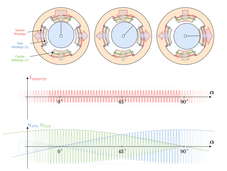
Switch Reluctance Motor

Based on a wikimedia image from Hamidreza D (CC-SA 4.0)