This is an old revision of the document!
7. Polyphase Networks and Power in AC Circuits
emphasizing the importance of power considerations
- three phase four wire systems
7.0 Recap of complex two-terminal networks
In the last semester, AC current, AC voltage and their effects have been considered on a circuit that had simply included a AC voltage source.
These circuits can be now understood as.
- the sinusoidal alternating voltage is produced by the rotation of a coil in a homogeneous magnetic field, and
- the sinusoidal alternating current is formed by a connected load (or complex impedance).
are formed.
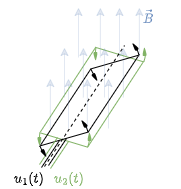
This will be briefly illustrated here. In figure 1 a coil with $w$ windings is seen in a magnetic field with a magnetic flux density $\vec{B}$. The coil rotates - starting from $\varphi_0$ with angular velocity $\omega$. The rotation changes the chained flux $\Psi$ through the coil and thus a voltage $u(t)$ is induced.

For the rotation angle $\varphi$ holds: \begin{align*} \varphi(t)=\omega t + \varphi_0 \quad \text{with} \quad \varphi_0=\varphi(t=0) \\ \end{align*}
Thus, the induced voltage $u(t)$ is given by: \begin{align*} u(t) &= \frac{d\Psi}{dt} \\ &= N\cdot\frac{d\Phi}{dt} \\ &= NBA\cdot\frac{d cos \varphi(t)}{dt} \\ &= \hat{\Psi}\cdot\frac{d cos (\omega t + \varphi_0)}{dt} \\ &= -\omega \hat{\Psi}\cdot sin (\omega t + \varphi_0) \\ &= -\hat{U}\cdot sin (\omega t + \varphi_0) \\ \end{align*}
Such single-phase systems are therefore alternating current systems, which use one outgoing line and one return line each for the current conduction.
Out of the last formula we derived the following instantaneous voltage $u(t)$ \begin{align*} u(t) &= -\hat{U}\cdot sin (\omega t + \varphi_0) \\ &= \hat{U}\cdot sin (\omega t + \varphi'_0) \\ &= \sqrt{2} U\cdot sin (\omega t + \varphi'_0) \\ \end{align*}
7.1 Power in AC
Learning Objectives
By the end of this section, you will be able to:
- Know the formula of the instantaneous power of the resistor, inductor and capacitor and be able to determine its values.
In the first chapter we mainly focussed on the power given by $P = U \cdot I$. This is however only valid for DC circuits. For AC circuits we have to consider the instantaneous power $p(t)$. The instantaneuos power is given by:
\begin{align*} p(t) &= \color{blue}{u(t)} \cdot \color{red}{i(t)} \end{align*}
Ideal Ohmic resistance R
The simplest component to look at for the instantaneuos power is the resistor. For this, we start with the basic definition of the instantaneous voltage $u_R(t)$ (which was given in the last semester) as
\begin{align*} \color{blue}{u_R(t)} &= \sqrt{2}U sin(\omega t + \varphi_u) \end{align*}
With the defining formula for the resistor we get:
\begin{align*} \color{blue}{u_R(t)} &= R \cdot \color{red}{i(t)} \\ \rightarrow \color{red}{i(t)} &= {{\color{blue}{u_R(t)}}\over{R}} \\ &= \sqrt{2} {{U}\over{R}} sin(\omega t + \varphi_u) \end{align*}
This leads to an instantaneous power $p_R(t)$ of
\begin{align*} p_R(t) &= \color{blue}{u_R(t)} \cdot \color{red}{i_R(t)} \\ &= 2\cdot {{U^2}\over{R}} sin^2(\omega t + \varphi_u) \\ &= {{U^2}\over{R}}\left(1- cos\left(2\cdot (\omega t + \varphi_u)\right)\right) \\ \end{align*}
For the last step the Double-angle formula “$cos(2x) = 1 - 2 sin^2(x)$” was used.
This result is interesting in the following ways:
- The part $1- cos (2\cdot (\omega t + \varphi_u) )$ is always non-negative and a shifted sinusidal function between $0...2$. The average value of this part is $1$.
- The average value of $p_R(t)$ is then: $P_R = {{U^2}\over{R}}$
- The use of the $\sqrt{2}$ in the definition $\color{blue}{u_R(t)} = \sqrt{2} U sin(\omega t + \varphi_u)$ leads to the average power as $P_R = {{U^2}\over{R}}$. This formula for the power is exactly like the formula for the power in pure DC situations.
Ideal Inductivity L
The similar approach is done for the inductivity. We again start with the basic definition of the instantaneous voltage
\begin{align*} \color{blue}{u_L(t)} &= \sqrt{2}U sin(\omega t + \varphi_u) \end{align*}
With the defining formula for the inductivity we get: \begin{align*} \color{blue}{u_L(t)} &= L\cdot {{d\color{red}{i_L(t)}}\over{dt}} \\ \rightarrow \color{red}{i_L(t)} &= {{1}\over{L}} \int \color{blue}{u_L(t)} dt \\ &= - \sqrt{2} {{U}\over{\omega L}} cos(\omega t + \varphi_u) \end{align*}
This leads to an instantaneous power $p_L(t)$ of
\begin{align*} p_L(t) &= \color{blue}{u(t)} \cdot \color{red}{i(t)} \\ &= - 2\cdot {{U^2}\over{\omega L}} \cdot sin(\omega t + \varphi_u) cos(\omega t + \varphi_u) \\ &= - {{U^2}\over{\omega L}} \cdot sin( 2\cdot (\omega t + \varphi_u)) \\ \end{align*}
Again a trigonometric identity (Double-angle formula “$sin(2x) = 2 sin(x)cos(x)$”) was used.
Also this result is interesting:
- The part $sin( 2\cdot (\omega t + \varphi_u))$ has an average value of $0$.
- Therefore, the average value of $p_L(t)=0$
Ideal Capacity C
Also here, we start with the basic definition of the instantaneous voltage
\begin{align*} \color{blue}{u_C(t)} &= \sqrt{2}U sin(\omega t + \varphi_u) \end{align*}
With the defining formula for the capacity we get: \begin{align*} \color{red}{i_C(t)} &= C {{d\color{blue}{u_C(t)}}\over{dt}} \\ &= \sqrt{2} U \omega C cos(\omega t + \varphi_u) \end{align*}
This leads to an instantaneous power $p_C(t)$ of
\begin{align*} p_C(t) &= \color{blue}{u_C(t)} \cdot \color{red}{i_C(t)} \\ &= 2\cdot U^2 \omega C \cdot sin(\omega t + \varphi_u) cos(\omega t + \varphi_u) \\ &= + U^2 \omega C \cdot sin( 2\cdot (\omega t + \varphi_u)) \\ \end{align*}
Again this result leads to:
- The part $sin( 2\cdot (\omega t + \varphi_u))$ has an average value of $0$.
- Therefore, also the average value of $p_C(t)=0$
- Instantaneuos values of power at $R$, $L$, $C$
- Active, reactive, apparent, and complex power
This effect can also be seen in the following simulation: The simulation shows three loads, all with an impedance of $|Z| = 1 k\Omega$. The diagram on top of each circuit shows the instantaneous voltage, current and power.
- Ohmic load: The instantaneous voltage is in phase with the instantaneous current. The instantaneous power is always non negative. The average power is $P=U^2/R = {{1}\over{2}} \hat{U}^2/R= {{1}\over{2}}(6V)^2/1k\Omega = 18mW$
- Inductive load: The voltage is ahead of the current. The phase angle is $+90°$ (which also reflects the $+j$ in the inductive impedance $+j\omega L$). The instantaneous is half positive, half negative; the average power is zero (in the simulation not completely visible).
- Capacitive load: The voltage is lagging the current. The phase angle is $-90°$ (which also reflects the $-j$ in the capacitive impedance ${{1}\over{j\omega C}}$). The instantaneous is again half positive, half negative; the average power is zero (in the simulation not completely visible).
arbitrary two-terminal Component
For an arbitrary component we do not have any defining formula. But, the $u(t)$ and $i(t)$ can generally be defined as:
\begin{align*} \color{blue}{u(t)} &= \sqrt{2}U sin(\omega t + \varphi_u) \\ \color{red }{i(t)} &= \sqrt{2}I sin(\omega t + \varphi_i) \\ \end{align*}
This leads to an instantaneous power $p(t)$ of
\begin{align*} p(t) &= \color{blue}{u(t)} \cdot \color{red}{i(t)} \\ &= 2\cdot UI sin(\omega t + \varphi_u) sin(\omega t + \varphi_i) \\ \end{align*}
The formula can be further simplified with the help of the following equations
- $\varphi = \varphi_u - \varphi_i \quad \rightarrow \varphi_i = \varphi_u - \varphi$
- $sin(\Box - \varphi) = sin(\Box) cos \varphi - cos(\Box) sin \varphi $
- $2sin\Box sin\Box = 1 - cos(2\Box)$
- $2sin\Box cos\Box = sin(2\Box)$
\begin{align*} p(t) = UI\big( cos\varphi \left( 1- cos(2(\omega t + \varphi_u)\right) - sin\varphi \cdot sin(2(\omega t + \varphi_u) \big) \\ \end{align*}
This result is twofold:
- The part $ cos\varphi \; \cdot \; \left( 1- cos(2(\omega t + \varphi_u)\right)$ results into a non-zero average - explicitly this part is $1$ in average. On average the first part of the formula result into $UI cos\varphi$.
- The part $- sin\varphi \; \cdot \; sin(2(\omega t + \varphi_u))$ is zero in average, so the second part of the formula result into zero. The amplitude of the second part is $UI sin\varphi$
Notice:
A distinction is now made between:- An active power (alternatively real or true power, in German: Wirkleistung): $P = UI cos \varphi$
- The active power represents a pulsed energy drain out of the electrical system (commonly by an ohmic resistor).
- The active power transform the electric energy permanently into thermal or mechanical energy
- Therefore, the unit of the active power is $Watt$.
- A reactive power (in German: Blindleistung): $Q = UI sin \varphi$
- The reactive power describes the “sloshing back and forth” of the energy into the electric and/or magnetic fields.
- The reactive power is completely regained by the electic circuit.
- In order to distinguish the values, the unit of the reactive power is $V\!\! Ar$ (or $Var$) for V olta mpere-r eactive.
- An apparent power (in German Scheinleistung): $S = UI $
- The apparent power is the simple multiplication of the RMS values from the current and the voltage.
- The apparent power shows only what seem to be a value of power, but can deviate from usable power, when indoctors aor capacitors are used in the circuit.
- The unit of the apparent power is $V\!\! A$ for V olta mpere
Similarly, the currents and voltages can be separated into active, reactive and apparent values.
Based on the given formulas the three types of power are connected with each other. Since the apparent power are given by $S=U\cdot I$, the active power $P = U\cdot I \cdot sin \varphi = S \cdot sin \varphi $ and the reactive power $Q = S \cdot cos \varphi $, the relationship can be shown in a triangle (see figure 2).

Generally, the apparent power can also be interpreted as a complex value:
\begin{align*} \underline{S} &= S \cdot e^{j\varphi} \\ &= U \cdot I \cdot e^{j\varphi} \end{align*}
Based on the definition of the phase angle $\varphi = \varphi_U - \varphi_I$, this can be divided into:
\begin{align*} \underline{S} &= U \cdot I \cdot e^{j(\varphi_U - \varphi_I)} \\ &= \underbrace{U \cdot e^{j\varphi_U}}_{\underline{U}} \cdot \underbrace{I \cdot e^{-j\varphi_I}}_{\underline{I}^*} \end{align*}
where $\underline{I}^*$ is the complex conjungated value of $\underline{I}$.
Notice:
The apparent power $\underline{S} $ is given by:- $\underline{S} = UI \cdot e^{j\varphi}$
- $\underline{S} = UI \cdot (cos\varphi + j sin\varphi)$
- $\underline{S} = P + jQ$
- $\underline{S} = \underline{U} \cdot \underline{I}^*$
The following simulation shows three ohmic-inductive loads, all with an impedance of $|Z| = 1 k\Omega$, however with different phase angles $\varphi$. The diagram on top of each circuit shows the instantaneous voltage, current and power. Similar to the last simulation, a pure ohmic resistance would consume an average power of $P=U^2/R = {{1}\over{2}} \hat{U}^2/R= {{1}\over{2}}(6V)^2/1k\Omega = 18mW$. The three diagrams shall be duscussed shortly
- Phase angle $\varphi = 10°$: Nearly all of the impedance id given by the resistance and therefore the real part of the impedance. The instantaneous voltage is nearly in phase with the current. The instantaneous power is almost always larger than zero. The average power with $17.47mW$ is about the same like for an ohmic impedance.
- Phase angle $\varphi = 60°$: It is clearly visible, that instantaneous voltage and current are out of phase. The instantaneous power is often lower than zero. The ohmic resistor has $500\Omega = {{1}\over{2}}|Z|$, but does not show half of the voltage! This is due to the fact that the addition has to respect the complex behavior of the values. The complex part is $90°$ perpendicular to the real part - so they generate a right-angled triangle. The average power with $9mW$ is exactly the half of the power for an ohmic impedance, since only the resistance provides a way for consuming power permanently.
- Phase angle $\varphi = 84.28°$: The phase angle is calculated in such a way, that the resistance is only 10% of the amplitude of the impedance $|Z|$. In this case load is nearly pure inductive. The instantaneous power is consequently almost half of the time lower than zero. The average power here also only $10%$ of the power for an pure ohmic impedance.
The next simulation enables to play around with the phase angle of an impedance. The circuit on the left side is a bit harder to understand, but consist of a resistive (real) impedance and an complex impedance, which are driven by an AC voltage source. All of these components are parameterizable in such a way that the phase angle can be manipulated by the slider on the right side.
In the middle part reflects the time course of:
- The instantaneous power $p$ of the real part (active power), the imaginary part (reactive power) and overall power.
- The instantaneous voltage and current.
On the right-hand side the impedance Phasor is shown (lower diagram). The upper diagram depicts the $u$-$i$-diagram, which would be a perfect line for an pure ohmic resistance (since $u_R = R \cdot i_R$) and a circle for a pure complex impedance (since the phase angle of $\pm 90°$ between $u_{L,C}$ and $i_{L,C}$). The simulation is in this part not completely perfect: The pure line and circle are sometimes not reachable.
The folllowing questions can be solved with this simulation:
- How does the amplitude of the active and reactive instantaneous power change, when the phase angle is changed between $-90°...+90°$?
- What is the phase shift between the active and reactive instantaneous power?
Also the last simulation shows the relation between the phase angle (here: $\alpha$) and instantaneous values, like power, voltage and current.
7.1.3 Applications
Power Factor Correction
Cables and components have to conduct the sum of active and reactive current, but only the active current is used outside of the circuit. Therefore, a common goal is to minimize the reactive part. The technical way to represent this the power factor $pf$ is used.
Notice:
The power factor is given by:\begin{align*} pf &= cos \varphi \\ &= {{P}\over{|\underline{S}|}} \end{align*}
The power factor shows how much real power one gets out of the needed apparent power.
How does the power factor show the problematic effects? For this one can investigate situation of a ohmic-inductive load $\underline{Z}_L$ which is connected to a voltage $\underline{U}_0$ source with a wire $R_{wire}$. This circuit is shown in figure 4.

The usable output power is $P_L = U_L \cdot I \cdot cos \varphi$. Based on this, the current $\underline{I}$ is:
\begin{align*} I = {{P_L}\over{U_L \cdot cos \varphi}} \end{align*}
The power loss of the wire $P_{wire}$ is therefore:
\begin{align*} P_{wire} &= R_{wire} \cdot I^2 \\ &= R_{wire} \cdot {{P_L^2}\over{U_L^2 \cdot cos^2 \varphi}} \end{align*}
This means: As smaller the power factor $cos \varphi$, as more power losses $P_{wire}$ will be generated. More power losses $P_{wire}$ leads to more heat up to or even beyond the maximum temperature. In order to compensate this, the cross section of the wire have to be increased, which means more copper.
Alternatively, a bad power factor the can be compensated with a counteracting complex impedance. This compensating impedance has to provide enough power with the opposite sign to cancel out the unwanted reactive power. The following simulation shows an uncompensated circuit and a circuit with power factor correction. In the ladder the voltage on the load resistor is the same, but the current provided by the power supply is smaller.
Another explanation of power factor can be seen here:
Impedance matching
not covered in this course
7.2 Polyphase Networks
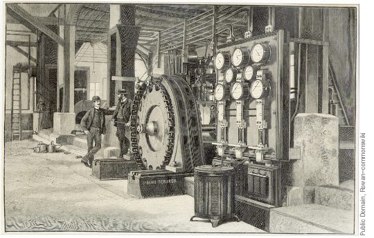
In order to transfer power over long distances alternating current ans explicitely rotary current is used. Rotary current is the common name for three-phase current. The first three-phase high Voltage power transfer worldwide started in the August of 1891 for the “International Electrotechnical Exhibition ”. The power plant in Lauffen (see figure 5) - about 10km away from the uinversity Heilbronn - was therefore the first modern three-phase generator and started the three-phase transimssion networks, which are the power backbone throughout the world.
In the following, the way to polyphase networks and explicitely three-phase systems will be described. Be aware, that the term “phase” is used in two different meanings: In the first usage, the phase shift $\varphi$ between voltage and current on a single component is commonly called “phase”. The second usage of “phase” is for a single circuit of a “multi circuit” setup, called polyphase network. The ladder terminology will be explained in the following in more detail.
7.2.1 Technical terms of the Polyphase Networks
General
Various general technical terms in the polyphase system (in German: Mehrphasensystem) will now be briefly discussed.
- A $m$-phase system describes a circuit in which $m$ sinusoidal voltages transport the power. The general term of these systems is polyphase systems.
The voltages are generated by a homogenous magnetic field containing $m$ rotating windings, which are arranged with a fixed offset to each other (see figure 6). The induced voltages exhibit the same frequency $f$.
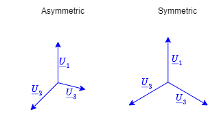
- An $m$-phase system is symmetrical when the voltages of the individual windings exhibit the same amplitude and are offset at the same angle to each other ($\varphi = 2\pi/m$).
Thus, the voltage phasors $\underline{U}_1 ... \underline{U}_m$ form a symmetrical star.
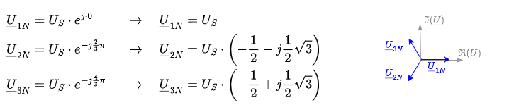
Example: A 3-phase system is symmetrical for $\varphi = 360°/3 = 120°$ beween the voltages of the windings: $\underline{U}_1 = \sqrt{2} \cdot U \cdot e ^{j(\omega t + 0°)}$, $\underline{U}_2 = \sqrt{2} \cdot U \cdot e ^{j(\omega t - 120°)}$, $\underline{U}_3 = \sqrt{2} \cdot U \cdot e ^{j(\omega t - 240°)}$
- The windings can be concatenated (=linked) in different ways. The most importend ways of concatenation are:
- All windings are independently connected to a load. This phase system is called non-interlinked (in German: nicht verkettet).
- All windings are connected to each other, then the phase system is called interlinked.
With interlinking, fewer wires are needed. Star or ring circuits can be used for daisy chaining.
The two simulations in figure 8 show a non-interlinked and an interlinked circuit with generator and load in star shape.
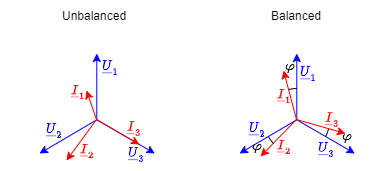
- The instantaneous power $p_i(t)$ of a winding $i$ is variable in time. For the instantaneous power $p(t)$ of the $m$-phase system one has to consider all single instantaneous powers of the windings. When this instantaneous power $p(t)$ does not change with time, the polyphase system is called balanced.
If a balanced load is used, then polyphase systems are balanced with $m\geq3$.
For $m\geq3$ and symmetrical load, the following is obtained for the instantaneous power:
$\quad \quad p = m \cdot U \cdot I \cdot cos\varphi = P$
The following simulation shows the power in the different phases of a symmetrical and balanced system. The instantaneous power of each phase is a non-negative sinusidal function shifted by $0°$, $120°$ and $240°$.
Balanced polyphase networks have the lowest wiring costs.
Polyphase networks are also possible in ring interlinking (also called ring connection, see next simulation).
The often used (and also here used) term of three-phase current or alternating current have not be taken literally: If no load is connected, there is no three-phase AC network, but a three-phase voltage network.
7.2.2 Three-Phase System
The most commonly used polyphase system is the three-phase system. The three-phase system has advantages over a DC system or single phase AC system:
- Simple three-phase machines can be used for generation.
- Rotary field machines (e.g. synchronous motors or induction motors) can also be simply connected to as load, converting the electrical energy into mechanical energy.
- When a symmetrical load can be assumed, the energy flow is constant in time.
- For energy transport, the voltage can be up-transformed and thus the AC current, as well as the associated power loss (= waste heat), can be reduced.
In order to understand the three-phase system, we have to investigate the different voltages and currents in this system.
For this the three-phase system will be separated into three parts:
- Three-phase generator(s)
- Line conductors
- Loads
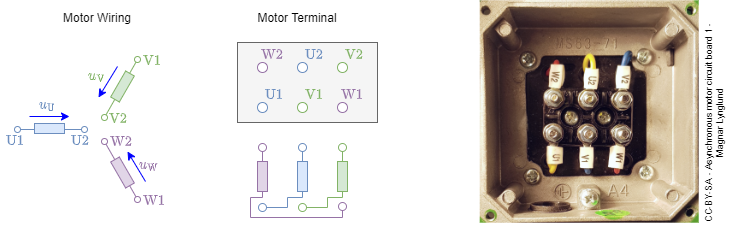
Three-phase generator
- The windings of a three-phase generator are called $U$, $V$, $W$; the winding connections are correspondingly called: $U1$, $U2$, $V1$, $V2$, $W1$, $W2$ (see figure 11).
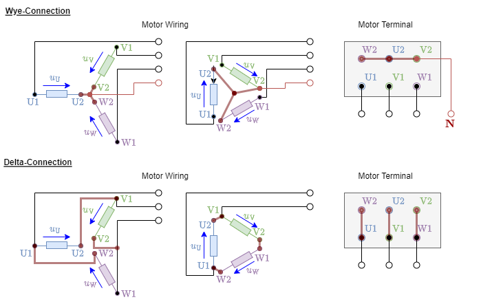
- The typical winding connections in a three-phase generator are called Delta connection (for ring connection) and Wye connection (for star connection). This winding connections can simply be changed by reconnecting the motor terminal. In figure 12 the two types of winding connections are shown. Often for Wye connection the star configuration is shown and for Delta connection the ring configuration. For Wye-connection is is also possible to have the star point on an separate terminal.
- The phase voltages are given by:
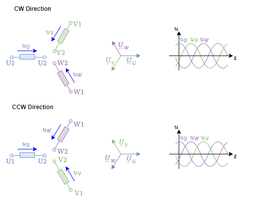
\begin{align*} \color{RoyalBlue}{u_U} &\color{RoyalBlue}{= \sqrt{2} U \cdot cos(\omega t + \alpha - 0)} \\ \color{Green}{u_V} & \color{Green}{= \sqrt{2} U \cdot cos(\omega t + \alpha - {{2}\over{3}}\pi)} \\ \color{DarkOrchid}{u_W} & \color{DarkOrchid}{= \sqrt{2} U \cdot cos(\omega t + \alpha - {{4}\over{3}}\pi)} \\ \color{RoyalBlue}{u_U} + \color{Green}{u_V} + \color{DarkOrchid}{u_W} & = 0 \end{align*} - The direction of rotation is given by the arrangement of the windings:
- The three-phase generator with clockwise direction (CW, mathematically negative orientation) shows the phase sequence: $u_U$, $u_V$, $u_W$, Therefore, $u_V$ is $120°$ lagging to $u_U$.
This is the common setup for generators. - The three-phase generator with counter-clockwise direction (CCW, mathematically positive orientation) shows the phase sequence: $u_U$, $u_W$, $u_V$, Therefore, $u_V$ is $120°$ ahead of $u_U$.
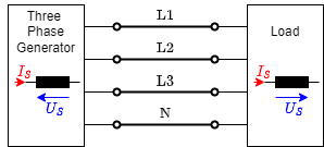
Line Conductors
The lines connected to the generator / load terminals $U1$, $V1$, $W1$ are often called $L1$, $L2$, $L3$ ($L$ for Line or Live = active) outside of the generator or load.
It is important to distinguish between the different types of voltages and currents, which depent on the point of view (either onto a three-phase generator/load or the external conductors).
- String voltages/currents $U_S$ (alternatively: winding voltages/currents, in German: Strangströme/Strangspannungen):
The string voltages/currents are the values measured on the windings - independent on the winding connection.
These voltages are shown in the previous images as $u_U$, $u_V$, $u_W$. - Phase voltages/currents $U_L$ (alternatively: phase-to-phase voltages/currents, line-to-line voltages/currents, external conductor voltages/currents, in German: Außenleiterströme/Außenleiterspannungen):
The phase voltages are measured differentially between the lines. The phase voltages are therefore given as $U_{12}$, $U_{23}$, $U_{31}$.
The phase currents are given as the currents through a single line: $I_1$, $I_2$, $I_3$.
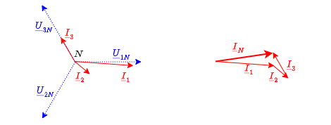
The potential of the star point is called neutral $N$ - Star voltages (alternatively: phase-to-neutral voltages, line-to-neutral voltages, in German: Sternspannungen): the voltages of the lines can be also measured or used refering to the neutral potential.
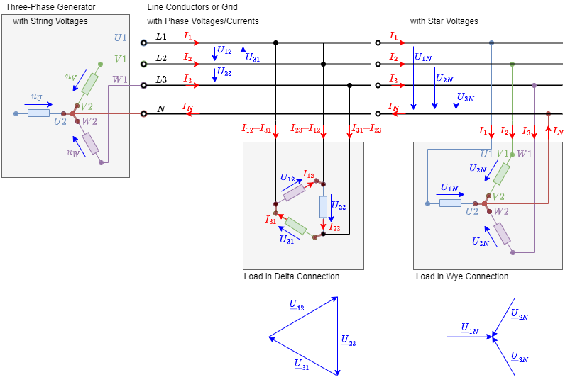
The setup with $L1$, $L2$, $L3$ and $N$ is called three-phase four-wire system. When only a Delta connection without neutral is connected it is called a three-phase three-wire system. The star and phase voltages are given by

A phasor diagram can be constructed based on the given voltages. Be aware, that commonly the phasor is shown as vector (i.e. as an arrow starting from the origin or zero). In contrast to this, the voltage in a circuit is shown as a arrow pointing towards the zero potential.
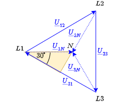
For the yellow triangle in figure 15 applies:
\begin{align*} {{1}\over{2}} U_{31} &= U_{1N} \cdot cos 30° \\ &= U_{1N} \cdot {{\sqrt{3}}\over{2}} \\ \\ U_{31} &= \sqrt{3} \cdot U_{1N} \\ U_{L} &= \sqrt{3} \cdot U_{S} \\ \end{align*}
The phase voltages are $\sqrt{3}$ larger than the star voltage. In Europe the low-voltage network of electric power distribution is defined by the RMS value of a star voltage of $400V$. The phase voltage is therefore ${{1}\over{\sqrt{3}}} \cdot 400V \approx 230V$. The following two simulations show these voltages.
7.2.3 Load and Power in Three-Phase Systems
In order to understand the load in three-phase systems, the power at different types of loads are investigated:
- Load in Wye connection with three-phase four-wire system
- Load in Wye connection with three-phase three-wire system
- Load in Delta connection
An example circuit is chosen for each investigation.
Load in Wye connection (Four-Wire System)
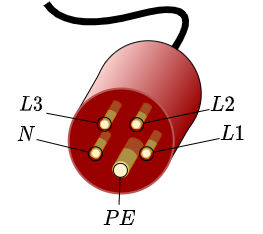
The four-wire wiring is one of the most common way to connect three-phase systems. The IEC 60309 connector (in German commonly knwon as CEE Stecker) is often used for this connection. The connector has an additional pin $PE$, besides the explained phases $L1$, $L2$, $L3$ and the neutral line $N$. PE stand for protective earth and is part of the Earthing System. In short: PE provides a reference potential, which is everywhere available, due to the fact, that the power plant provide it to the soil ground.
For the four-wire system, the four pins $L1$, $L2$, $L3$ and the neutral line $N$ are used for power transfer. This is for example applied for loads in star configuration, e.g. three-phase motors in Wye connection or three one phase loads, where each load is connected ot a single phase.
Example
The example in the following simulation shows a $50Hz$ / $231V$ three-phase four-wire system with unbalanced load in Wye connection, with the given impedances.
- Calculate the phase currents $I_1$, $I_2$, $I_3$, the neutral current $I_N$
- Calculate the true power, apparent power and reactive power.
Voltages - Currents - True Power - Aparrent and Reactive Power
The following “path”: calculate voltages $\rightarrow$ calculate currents $\rightarrow$ calculate true power $\rightarrow$ calculate aparrent and reactive power is the best way to get to all wanted values.
- Voltages: It is obvious, that the phase voltages $U_L$ and star voltages $U_S$ are applied by the three-phase network independently of the load.
- Currents: For the phase currents it applies that: $\underline{I}_1 + \underline{I}_2 + \underline{I}_3 = \underline{I}_N $ (be aware, that the voltage given in the simulation is only the RMS value without the phase shift).
The phase currents are given by the phase impedances and the star voltages:
\begin{align*} \underline{I}_1 = {{\underline{U}_{1N}}\over{\underline{Z}_1^\phantom{O}}} \quad , \quad \underline{I}_2 = {{\underline{U}_{2N}}\over{\underline{Z}_2^\phantom{O}}} \quad , \quad \underline{I}_3 = {{\underline{U}_{3N}}\over{\underline{Z}_3^\phantom{O}}} \\ \end{align*} - The true power $P_x$ for each string is given by the apparent power $S_x$ of the string times the indivitual phase angle $\varphi_x$ of the string:
\begin{align*} P_x &= S_x \cdot cos \varphi_x = U_S \cdot I_x \cdot cos \varphi_x \end{align*}
Therefore, the resulting true power for the full load is:
\begin{align*} P = U_S \cdot ( I_1 \cdot cos \varphi_1 + I_2 \cdot cos \varphi_2 + I_3 \cdot cos \varphi_3) \end{align*}
The angle $\varphi$ here is given by $\varphi = \varphi_u - \varphi_i$, and hence:
\begin{align*} P = U_S \cdot \left( I_1 \cdot cos (\varphi_{u,1} - \varphi_{i,1})+ I_2 \cdot cos (\varphi_{u,2} - \varphi_{i,2}) + I_3 \cdot cos (\varphi_{u,3} - \varphi_{i,3})\right) \end{align*} - For the apparent power one could think of $S_x$ for each string is given by the string voltage and the current through the string $S_x = U_S \cdot I_x$. However, this misses out the apparent power of the neutral line!
Even when considering all four lines a simple addition of all the apparent powers per phase would be problematic: The apparent power can be either positive or negative. There is the possibility to chancel each other out in the calculation, even when there is an unbalanced impedance given. It is better to use a definition, which can consider all of phase apparent powers.
By DIN 40110 the collective apparent power $S_\Sigma$ can be assumed as
\begin{align*} S_\Sigma &= \sqrt{\sum_x U_{x N}^2+ \underbrace{U_N^2}_{=0}} &\cdot & \sqrt{\sum_x I_{x}^2+ I_N^2} \\ &=\sqrt{3} \cdot U_S & \cdot & \sqrt{I_1^2 + I_2^2 + I_2^3 + I_N^2} \\ \end{align*} - Given the collective apparent power the collective reactive power $Q_\Sigma$ ist given by
\begin{align*} Q_\Sigma = \sqrt{S_\Sigma^2-P^2} \end{align*}
Example
In the example this leads to:
- The star voltages and the phase voltages are given as \begin{align*} U_S=& 231V = U_{1N} = U_{2N} = U_{3N} \\ U_L=\sqrt{3} \cdot 231V = & 400V = U_{12} = U_{23} = U_{31} \end{align*}
The phasors of the star voltages are given as:
- Based on the star voltages and the given impedances the phase currents are:
\begin{align*} \underline{I}_1 &= {{\underline{U}_{1N}}\over{\underline{Z}_1}} &= &{{231V}\over{10\Omega + j \cdot 2\pi\cdot 50Hz \cdot 1mH}} &= &+23.08 A &- j \cdot 0.72 A &= &23.08 A \quad &\angle -1.8° \\ \underline{I}_2 &= {{\underline{U}_{2N}}\over{\underline{Z}_2}} &= &{{231V \cdot \left( -{{1}\over{2}}-j{{1}\over{2}}\sqrt{3}\right)}\over{5\Omega + {{1}\over{j \cdot 2\pi\cdot 50Hz \cdot 100\mu F}}}} &= &+ 5.58 A &- j \cdot 4.50 A &= & 7.17 A \quad &\angle -38.9° \\ \underline{I}_3 &= {{\underline{U}_{3N}}\over{\underline{Z}_3}} &= &{{231V\cdot \left( -{{1}\over{2}}+j{{1}\over{2}}\sqrt{3}\right)}\over{20 \Omega}} &= &-5.78A &+ j \cdot 10.00A &= &11.55 A \quad &\angle -240.0° \\ \\ \underline{I}_N & = \underline{I}_1 + \underline{I}_2 + \underline{I}_3 & & & = &+22.88 A &+ j \cdot 4.77 A &= &23.37 A \quad &\angle +11.8° \end{align*} - The true power is calculated by:
\begin{align*} P = 231V \cdot \big( 23.08 A \cdot cos (0° - (-1.8°))+ 7.17A \cdot cos (-120° - (-38.9°)) + 11.55 A \cdot cos (-240° - (-240°)\big) = 8.26 kW \end{align*} - The collective apparent power is:
\begin{align*} S_\Sigma &=\sqrt{3} \cdot 231V & \cdot & \sqrt{(11.54A)^2 + (7.17A)^2 + (11.54A)^3 + (12.53A)^2} = 14.23 kVA \\ \end{align*} - The collective reactive power is:
\begin{align*} Q_\Sigma &=\sqrt{(8.72 kVA)^2 - (5.59 kW)^2} = 11.58kVar \\ \end{align*}
For Symmetric Load
In case of a symmetric load the situation and the formulas get much simplier:
- The phase voltages $U_L$ and star voltages $U_S$ are equal to the asymmetric load: $U_L = \sqrt{3}\cdot U_S$.
- For equal impedances the absolute value of all phase currents $I_x$ are the same: $|\underline{I}_x|= |\underline{I}_S| = {{\underline{U}_S}\over{\underline{Z}_S^\phantom{O}}}$. Since the phase currents the same absolute value and have the same $\varphi$, they will add up to zero. Therefore there is no current on neutral line: $I_N =0$
- The true power is three times the true power of a single phase: $P = 3 \cdot U_S I_S \cdot cos \varphi$. Based on the line voltages $U_L$, the formula is $P = \sqrt{3} \cdot U_S I_S \cdot cos \varphi$
- The (collective) apparent power - given the formula above - is: $S_\Sigma = \sqrt{3}\cdot U_S \cdot \sqrt{3\cdot I_S^2} = 3 \cdot U_S I_S$. This corresponds to three times the apaarent power of a single phase.
- The reactive power leads to: $Q_\Sigma = \sqrt{S_\Sigma^2 - P^2} = 3 \cdot U_S I_S \cdot sin (\varphi)$.
Load in Wye connection with (Three-Wire System)
The three-wire system is used the four pins $L1$, $L2$, $L3$ and the neutral line $N$ are used for power transfer.
Sometimes the load do not provide a neutral connection, even when it is in Wye connection - the star point can for example only be provided for measurement with a thin cable.
Additionally, the neutral connection of a load in Wye connection can break an lead to a three wire system.
In the case of three wire system, only the potentials $L1$, $L2$ and $L3$ are provided and used for power transfer.
Example
The example in the following simulation shows a $50Hz$ / $231V$ three-phase three-wire system with unbalanced load in Wye connection, with the given impedances.
- Calculate the phase currents $I_1$, $I_2$, $I_3$, the neutral current $I_N$
- Calculate the true power, apparent power and reactive power.
The following simulation has the same impedances in the load, but the load does not provide a neutral connection.
Voltages - Currents - True Power - Aparrent and Reactive Power
The simulation differs in the following:
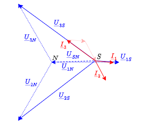
- The network star voltages $\underline{U}_{1N}$, $\underline{U}_{2N}$, $\underline{U}_{3N}$ related to the neutral potential $\underline{U}_N$, and the load star voltages $\underline{U}_{1S}$, $\underline{U}_{2S}$, $\underline{U}_{3S}$ related to the star potential of the load are separated.
- The star point voltage $\underline{U}_{KN}$ is shown.
- With the switch $S$, the star potential can short-circuited to the neutral potential; so set $\underline{U}_{KN}=0$. This enables a comparison with the previous four-wire three-phase system.
Also here the “path”: calculate voltages $\rightarrow$ calculate currents $\rightarrow$ calculate true power $\rightarrow$ calculate aparrent and reactive power is the best way to get to all wanted values.
- Voltages: Here, only the the phase voltages $U_L$ are applied by the three-phase net, independently of the load. The star voltages of the load $\underline{U}_{xS}$ are not given by the network anymore, since the neutral potential is not provided. The network star voltages and the load star voltages can be connected in the following way: The calculation of the star voltage $\underline{U}_{SN}$ is explained after investigating the currents.
\begin{align*} \underline{U}_{1S} &= \underline{U}_{1N} - \underline{U}_{SN} \\ \underline{U}_{2S} &= \underline{U}_{2N} - \underline{U}_{SN} \\ \underline{U}_{3S} &= \underline{U}_{3N} - \underline{U}_{SN} \\ \end{align*} - Currents: For the phase currents it applies that: $\underline{I}_1 + \underline{I}_2 + \underline{I}_3 = 0$ (again, voltages given in the simulation are only the RMS value without the phase shift).
The phase currents are given by the phase impedances and the star voltages:
\begin{align*} \underline{I}_1 = {{\underline{U}_{1S}}\over{\underline{Z}_1^\phantom{O}}} \quad , \quad \underline{I}_2 = {{\underline{U}_{2S}}\over{\underline{Z}_2^\phantom{O}}} \quad , \quad \underline{I}_3 = {{\underline{U}_{3S}}\over{\underline{Z}_3^\phantom{O}}} \end{align*}
In order to get $\underline{U}_{SN}$, one has to combine the individual formulas for $\underline{I}_x$, $\underline{U}_{xS}$ and that the $\sum_x \underline{I}_x =0$. This leads to
\begin{align*} \underline{U}_{SN} = {{\sum_x \left( \Large{{{1}\over{\underline{Z}_x^\phantom{O}}}} \cdot \normalsize{\underline{U}_{xN}} \right) }\over{\sum_x \left( \Large{{{1}\over{\underline{Z}_x^\phantom{O}}}} \right) }} \end{align*} - Also here, the true power $P_x$ for each string is given by:
\begin{align*} P_x &= S_x \cdot cos \varphi_x = U_S \cdot I_x \cdot cos \varphi_x \end{align*}
Also here, the resulting true power for the full load is (with $U_S$ as the RMS value of the network star voltage):
\begin{align*} P &= U_S \cdot ( I_1 \cdot cos \varphi_1 + I_2 \cdot cos \varphi_2 + I_3 \cdot cos \varphi_3) \\ &= U_S \cdot \left( I_1 \cdot cos (\varphi_{u,1} - \varphi_{i,1})+ I_2 \cdot cos (\varphi_{u,2} - \varphi_{i,2}) + I_3 \cdot cos (\varphi_{u,3} - \varphi_{i,3})\right) \end{align*} - Since the three-wire system has no current out of the network star point, the apparent power $\underline{S}_x$ for each string is given by the string voltage and the current through the string $\underline{S}_x = \underline{U}_{xS} \cdot \underline{I}_x^*$. This leads to an overall apparent power $\underline{S}$ of
\begin{align*} \underline{S} &= P + j\cdot Q = \sum_x \underline{S}_x = \sum_x \left( \underline{U}_{xS} \cdot \underline{I}_x^* \right) \end{align*}
In order to simplify the calculation, it would be better to have a formula based on the network star voltages:
\begin{align*} \underline{S} &= \sum_x \left( \underline{U}_{xN} \cdot \underline{I}_x^* \right) + \underline{U}_{xN} \cdot \underbrace{\underline{I}_N}_{=0} \\ &= \sum_x \left( \underline{U}_{xN} \cdot \underline{I}_x^* \right) \\ \end{align*} Given that $\sum_x \underline{I}_x =0$, it is also true, that $\sum_x \underline{I}_x^* =0$ and so $\underline{I}_3^* = -\underline{I}_1^* - \underline{I}_2^*$.
By this, one can further simplify the calculation for the apparent power down to:
\begin{align*} \underline{S} &= \underline{U}_{13} \cdot \underline{I}_1^* + \underline{U}_{23} \cdot \underline{I}_2^* \\ &= \underline{U}_{12} \cdot \underline{I}_1^* + \underline{U}_{32} \cdot \underline{I}_3^* \\ &= \underline{U}_{21} \cdot \underline{I}_2^* + \underline{U}_{31} \cdot \underline{I}_3^* \end{align*}
For the phase voltages it applies that: $\underline{U}_{12} = - \underline{U}_{21}$, $\underline{U}_{23} = - \underline{U}_{32}$, $\underline{U}_{31} = - \underline{U}_{13}$. For the collective apparent power $S_\Sigma$ the formula of the four-wire system can be applied:
\begin{align*} S_\Sigma &= \sqrt{\sum_x U_{xN}^2} \cdot \sqrt{\sum_x I_x^2} &= \sqrt{3} U_S \cdot \sqrt{\sum_x I_x^2} \end{align*} - The abolute reactive power $Q$ can be calulated by the apparent power:
\begin{align*} j\cdot Q &= \underline{S} - P \end{align*}
the collective reactive power $Q_\Sigma$ is given by the collective apparent power:
\begin{align*} Q &= \sqrt{S_\Sigma^2 - P^2} \end{align*}
Example
In the example this leads to:
- The phase voltages are given as \begin{align*} U_L=\sqrt{3} \cdot 231V = & 400V = U_{12} = U_{23} = U_{31} \end{align*}
The phasors of the star voltages of the network are again given as:
- Based on the star voltages of the network and the given impedances the star voltage $\underline{U}_{SN}$ of the load can be calculated with :
\begin{align*} \underline{U}_{SN} = {{\sum_x \left( \Large{{{1}\over{\underline{Z}_x^\phantom{O}}}} \cdot \normalsize{\underline{U}_{xN}} \right) }\over{\sum_x \left( \Large{{{1}\over{\underline{Z}_x^\phantom{O}}}} \right) }} \end{align*}
Once investigating the numerator $\sum_x \big( {{1}\over{\underline{Z}_x^\phantom{O}}} \cdot \underline{U}_{xN} \big)$, once can see, that it just equals the sum of the phase currents of the four-wire system. So, the numerator equals the (in the three-wire system: fictive) current on the neutral line.
The numerator is therefore: $22.88A + j \cdot 4.77A$ (see calculation for the four-wire system).
The denominator is:
\begin{align*} \sum_x {{1}\over{\underline{Z}_x^\phantom{O}}} &= {{1}\over{10\Omega + j \cdot 2\pi\cdot 50Hz \cdot 1mH }} + {{1}\over{5\Omega + {{1}\over{j \cdot 2\pi\cdot 50Hz \cdot 100\mu F }} }}+ {{1}\over{20\Omega }} \\ \\ &= 0.1547 \cdot 1/\Omega + j \cdot 0.02752 \cdot 1/\Omega \end{align*}
The star voltage $\underline{U}_{SN}$ of the load is: \begin{align*} \underline{U}_{SN} &= {{22.88A + j \cdot 4.77A}\over{0.1547 \cdot 1/\Omega + j \cdot 0.0275 \cdot 1/\Omega}} \\ \\ &= 148.7V + j \cdot 4.41 V \end{align*}
Given this star voltage $\underline{U}_{SN}$ of the load, the phase currents are:
\begin{align*} \underline{I}_1 &= {{\underline{U}_{1N} - \underline{U}_{SN}}\over{\underline{Z}_1^\phantom{O}}} & = & {{231V - 148.7V - j \cdot 4.41 V}\over{10\Omega + j \cdot 2\pi\cdot 50Hz \cdot 1mH }} & = & +8.21A - j \cdot 0.70A &=& 8.24 A \quad \angle -4.9° \\ \underline{I}_2 &= {{\underline{U}_{2N} - \underline{U}_{SN}}\over{\underline{Z}_2^\phantom{O}}} & = & {{231V \cdot \left( -{{1}\over{2}}-j{{1}\over{2}}\sqrt{3}\right) - 148.7V - j \cdot 4.41 V}\over{5\Omega + {{1}\over{j \cdot 2\pi\cdot 50Hz \cdot 100\mu F }}}} & = & +5.00A + j \cdot 9.08A & =& 10.36 A \quad \angle -61.2° \\ \underline{I}_3 &= {{\underline{U}_{3N} - \underline{U}_{SN}}\over{\underline{Z}_3^\phantom{O}}} & = & {{231V \cdot \left( -{{1}\over{2}}+j{{1}\over{2}}\sqrt{3}\right) - 148.7V - j \cdot 4.41 V}\over{20\Omega }} &= & -13.21A + j \cdot 9.78A & =& 16.44A \quad \angle +143.5° \end{align*}
- The true power is calculated by:
\begin{align*} P = 231V \cdot \big( 8.24 A \cdot cos (0° - (-4.9°))+ 10.36A \cdot cos (-120° - (-61.2°)) + 16.44 A \cdot cos (-240° - (+143.5°)\big) = 6.62 kW \end{align*} - The apparent power $\underline{S}$ is:
\begin{align*} \underline{S} &= \underline{U}_{13} \cdot \underline{I}_1^* + \underline{U}_{23} \cdot \underline{I}_2^* &=& 400V \cdot (- e^{-j \cdot 7/6 \pi} \cdot (8.21 A + j \cdot 0.70 A ) + e^{- j \cdot 3/6 \pi} \cdot (5.00A - j \cdot 9.08A) ) &= 6.62 kW - j \cdot 3.40 kVAr \\ &= \underline{U}_{12} \cdot \underline{I}_1^* + \underline{U}_{32} \cdot \underline{I}_3^* &=& 400V \cdot (e^{j \cdot 1/6 \pi} \cdot (8.21A + j \cdot 0.70A) - e^{-j \cdot 3/6 \pi} \cdot (-13.21A -j \cdot 9.78A)) &= 6.62 kW - j \cdot 3.40 kVAr \\ &= \underline{U}_{21} \cdot \underline{I}_2^* + \underline{U}_{31} \cdot \underline{I}_3^* &=& 400V \cdot (- e^{j \cdot 1/6 \pi} \cdot (5.00A - j \cdot 9.08A) + e^{- j \cdot 7/6 \pi} \cdot (-13.21A - j \cdot 9.78A)) &= 6.62 kW - j \cdot 3.40 kVAr \\ & = 7.44 kVA \quad \angle -27.2°\end{align*}
The collective apparent power is:
\begin{align*} S_\Sigma &= \sqrt{3} U_S \cdot \sqrt{\sum_x I_x^2} \\ &= \sqrt{3} \cdot 231V \cdot \sqrt{(8.24A)^2+(10.36A)^2+(16.44A)^2} = 8.45 kVA \end{align*} - The reactive power is: \begin{align*} Q &= \underline{S} - P = -3.40kVAr \\ \end{align*}
The collective reactive power is:
\begin{align*} Q_\Sigma &=\sqrt{(8.44 kVA)^2 - (6.62 kW)^2} = 5.24kVAr \\ \end{align*}
For Symmetric Load
The case of a symmetric load in a three-wire system equals the symmetric load in a four-wire system, since the symmetric four-wire system also does not show a current on the neutral line.
Load in Delta connection
The delta connection uses also a three-wire system like the Wye connection without the neutral line.
Internally, the load is now connected in a triangluar shape. Therefore the individual string currents differ from the individual phase currents.
This setup is for example given for motors, when higher torque is needed. In this connection each string sees $U_L = \sqrt{3}\cdot U_S$ and can therefore produce more current and more power.
In the case of delct connection, also only the potentials $L1$, $L2$ and $L3$ are provided and used for power transfer.
Example
The example in the following simulation shows a $50Hz$ / $231V$ three-phase three-wire system with unbalanced load in delta connection, with the given impedances.
- Calculate the phase currents $I_1$, $I_2$, $I_3$, the neutral current $I_N$
- Calculate the true power, apparent power and reactive power.
The following simulation has the same impedances in the load, but the load does not provide a neutral connection.
Voltages - Currents - True Power - Aparrent and Reactive Power
The simulation differs in the following:
- The strings of the load are now connected to two phases and not to a star point anymore.
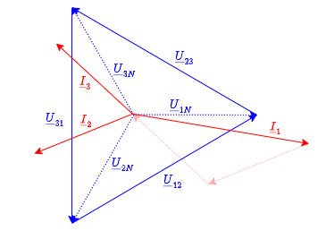
- The network phase voltages $\underline{U}_{12}$, $\underline{U}_{23}$, $\underline{U}_{31}$ equals to the string voltages of the load.
- The star point that the voltages toward is is here not relevant, and cannot be connected in any way to the strings.
Again here the “path”: calculate voltages $\rightarrow$ calculate currents $\rightarrow$ calculate true power $\rightarrow$ calculate aparrent and reactive power is the best way to get to all wanted values.
- Voltages: Here, the string voltages of the load are applied by the three phase net:
\begin{align*} \underline{U}_{12} = U_L \cdot e^{j\cdot {{1}\over{6}} \\ \underline{U }_{12} = U_L \cdot e^{- j\cdot {{3}\over{6}} \\ \underline{U }_{12} = U_L \cdot e^{- j\cdot {{7}\over{6}} \end{align*} - Currents: For the phase currents one can focus on the nodes it applies that: $\underline{I}_1 + \underline{I}_2 + \underline{I}_3 = 0$ (again, voltages given in the simulation are only the RMS value without the phase shift).
The phase currents are given by the phase impedances and the star voltages:
\begin{align*} \underline{I}_1 = {{\underline{U}_{1S}}\over{\underline{Z}_1^\phantom{O}}} \quad , \quad \underline{I}_2 = {{\underline{U}_{2S}}\over{\underline{Z}_2^\phantom{O}}} \quad , \quad \underline{I}_3 = {{\underline{U}_{3S}}\over{\underline{Z}_3^\phantom{O}}} \end{align*}
In order to get $\underline{U}_{SN}$, one has to combine the individual formulas for $\underline{I}_x$, $\underline{U}_{xS}$ and that the $\sum_x \underline{I}_x =0$. This leads to
\begin{align*} \underline{U}_{SN} = {{\sum_x \left( \Large{{{1}\over{\underline{Z}_x^\phantom{O}}}} \cdot \normalsize{\underline{U}_{xN}} \right) }\over{\sum_x \left( \Large{{{1}\over{\underline{Z}_x^\phantom{O}}}} \right) }} \end{align*} - Also here, the true power $P_x$ for each string is given by:
\begin{align*} P_x &= S_x \cdot cos \varphi_x = U_S \cdot I_x \cdot cos \varphi_x \end{align*}
Also here, the resulting true power for the full load is (with $U_S$ as the RMS value of the network star voltage):
\begin{align*} P &= U_S \cdot ( I_1 \cdot cos \varphi_1 + I_2 \cdot cos \varphi_2 + I_3 \cdot cos \varphi_3) \\ &= U_S \cdot \left( I_1 \cdot cos (\varphi_{u,1} - \varphi_{i,1})+ I_2 \cdot cos (\varphi_{u,2} - \varphi_{i,2}) + I_3 \cdot cos (\varphi_{u,3} - \varphi_{i,3})\right) \end{align*} - Since the three-wire system has no current out of the network star point, the apparent power $\underline{S}_x$ for each string is given by the string voltage and the current through the string $\underline{S}_x = \underline{U}_{xS} \cdot \underline{I}_x^*$. This leads to an overall apparent power $\underline{S}$ of
\begin{align*} \underline{S} &= P + j\cdot Q = \sum_x \underline{S}_x = \sum_x \left( \underline{U}_{xS} \cdot \underline{I}_x^* \right) \end{align*}
In order to simplify the calculation, it would be better to have a formula based on the network star voltages:
\begin{align*} \underline{S} &= \sum_x \left( \underline{U}_{xN} \cdot \underline{I}_x^* \right) + \underline{U}_{xN} \cdot \underbrace{\underline{I}_N}_{=0} \\ &= \sum_x \left( \underline{U}_{xN} \cdot \underline{I}_x^* \right) \\ \end{align*} Given that $\sum_x \underline{I}_x =0$, it is also true, that $\sum_x \underline{I}_x^* =0$ and so $\underline{I}_3^* = -\underline{I}_1^* - \underline{I}_2^*$.
By this, one can further simplify the calculation for the apparent power down to:
\begin{align*} \underline{S} &= \underline{U}_{13} \cdot \underline{I}_1^* + \underline{U}_{23} \cdot \underline{I}_2^* \\ &= \underline{U}_{12} \cdot \underline{I}_1^* + \underline{U}_{32} \cdot \underline{I}_3^* \\ &= \underline{U}_{21} \cdot \underline{I}_2^* + \underline{U}_{31} \cdot \underline{I}_3^* \end{align*}
For the phase voltages it applies that: $\underline{U}_{12} = - \underline{U}_{21}$, $\underline{U}_{23} = - \underline{U}_{32}$, $\underline{U}_{31} = - \underline{U}_{13}$. For the collective apparent power $S_\Sigma$ the formula of the four-wire system can be applied:
\begin{align*} S_\Sigma &= \sqrt{\sum_x U_{xN}^2} \cdot \sqrt{\sum_x I_x^2} &= \sqrt{3} U_S \cdot \sqrt{\sum_x I_x^2} \end{align*} - The abolute reactive power $Q$ can be calulated by the apparent power:
\begin{align*} j\cdot Q &= \underline{S} - P \end{align*}
the collective reactive power $Q_\Sigma$ is given by the collective apparent power:
\begin{align*} Q &= \sqrt{S_\Sigma^2 - P^2} \end{align*}
Example
In the example this leads to:
- The phase voltages are given as \begin{align*} U_L=\sqrt{3} \cdot 231V = & 400V = U_{12} = U_{23} = U_{31} \end{align*}
The phasors of the star voltages of the network are again given as:
- Based on the star voltages of the network and the given impedances the star voltage $\underline{U}_{SN}$ of the load can be calculated with :
\begin{align*} \underline{U}_{SN} = {{\sum_x \left( \Large{{{1}\over{\underline{Z}_x^\phantom{O}}}} \cdot \normalsize{\underline{U}_{xN}} \right) }\over{\sum_x \left( \Large{{{1}\over{\underline{Z}_x^\phantom{O}}}} \right) }} \end{align*}
Once investigating the numerator $\sum_x \big( {{1}\over{\underline{Z}_x^\phantom{O}}} \cdot \underline{U}_{xN} \big)$, once can see, that it just equals the sum of the phase currents of the four-wire system. So, the numerator equals the (in the three-wire system: fictive) current on the neutral line.
The numerator is therefore: $22.88A + j \cdot 4.77A$ (see calculation for the four-wire system).
The denominator is:
\begin{align*} \sum_x {{1}\over{\underline{Z}_x^\phantom{O}}} &= {{1}\over{10\Omega + j \cdot 2\pi\cdot 50Hz \cdot 1mH }} + {{1}\over{5\Omega + {{1}\over{j \cdot 2\pi\cdot 50Hz \cdot 100\mu F }} }}+ {{1}\over{20\Omega }} \\ \\ &= 0.1547 \cdot 1/\Omega + j \cdot 0.02752 \cdot 1/\Omega \end{align*}
The star voltage $\underline{U}_{SN}$ of the load is: \begin{align*} \underline{U}_{SN} &= {{22.88A + j \cdot 4.77A}\over{0.1547 \cdot 1/\Omega + j \cdot 0.0275 \cdot 1/\Omega}} \\ \\ &= 148.7V + j \cdot 4.41 V \end{align*}
Given this star voltage $\underline{U}_{SN}$ of the load, the phase currents are:
\begin{align*} \underline{I}_1 &= {{\underline{U}_{1N} - \underline{U}_{SN}}\over{\underline{Z}_1^\phantom{O}}} & = & {{231V - 148.7V - j \cdot 4.41 V}\over{10\Omega + j \cdot 2\pi\cdot 50Hz \cdot 1mH }} & = & +8.21A - j \cdot 0.70A &=& 8.24 A \quad \angle -4.9° \\ \underline{I}_2 &= {{\underline{U}_{2N} - \underline{U}_{SN}}\over{\underline{Z}_2^\phantom{O}}} & = & {{231V \cdot \left( -{{1}\over{2}}-j{{1}\over{2}}\sqrt{3}\right) - 148.7V - j \cdot 4.41 V}\over{5\Omega + {{1}\over{j \cdot 2\pi\cdot 50Hz \cdot 100\mu F }}}} & = & +5.00A + j \cdot 9.08A & =& 10.36 A \quad \angle -61.2° \\ \underline{I}_3 &= {{\underline{U}_{3N} - \underline{U}_{SN}}\over{\underline{Z}_3^\phantom{O}}} & = & {{231V \cdot \left( -{{1}\over{2}}+j{{1}\over{2}}\sqrt{3}\right) - 148.7V - j \cdot 4.41 V}\over{20\Omega }} &= & -13.21A + j \cdot 9.78A & =& 16.44A \quad \angle +143.5° \end{align*}
- The true power is calculated by:
\begin{align*} P = 231V \cdot \big( 8.24 A \cdot cos (0° - (-4.9°))+ 10.36A \cdot cos (-120° - (-61.2°)) + 16.44 A \cdot cos (-240° - (+143.5°)\big) = 6.62 kW \end{align*} - The apparent power $\underline{S}$ is:
\begin{align*} \underline{S} &= \underline{U}_{13} \cdot \underline{I}_1^* + \underline{U}_{23} \cdot \underline{I}_2^* &=& 400V \cdot (- e^{-j \cdot 7/6 \pi} \cdot (8.21 A + j \cdot 0.70 A ) + e^{- j \cdot 3/6 \pi} \cdot (5.00A - j \cdot 9.08A) ) &= 6.62 kW - j \cdot 3.40 kVAr \\ &= \underline{U}_{12} \cdot \underline{I}_1^* + \underline{U}_{32} \cdot \underline{I}_3^* &=& 400V \cdot (e^{j \cdot 1/6 \pi} \cdot (8.21A + j \cdot 0.70A) - e^{-j \cdot 3/6 \pi} \cdot (-13.21A -j \cdot 9.78A)) &= 6.62 kW - j \cdot 3.40 kVAr \\ &= \underline{U}_{21} \cdot \underline{I}_2^* + \underline{U}_{31} \cdot \underline{I}_3^* &=& 400V \cdot (- e^{j \cdot 1/6 \pi} \cdot (5.00A - j \cdot 9.08A) + e^{- j \cdot 7/6 \pi} \cdot (-13.21A - j \cdot 9.78A)) &= 6.62 kW - j \cdot 3.40 kVAr \\ & = 7.44 kVA \quad \angle -27.2°\end{align*}
The collective apparent power is:
\begin{align*} S_\Sigma &= \sqrt{3} U_S \cdot \sqrt{\sum_x I_x^2} \\ &= \sqrt{3} \cdot 231V \cdot \sqrt{(8.24A)^2+(10.36A)^2+(16.44A)^2} = 8.45 kVA \end{align*} - The reactive power is: \begin{align*} Q &= \underline{S} - P = -3.40kVAr \\ \end{align*}
The collective reactive power is:
\begin{align*} Q_\Sigma &=\sqrt{(8.44 kVA)^2 - (6.62 kW)^2} = 5.24kVAr \\ \end{align*}
For Symmetric Load
The case of a symmetric load in a three-wire system equals the symmetric load in a four-wire system, since the symmetric four-wire system also does not show a current on the neutral line.
Excercises
Exercise 7.1.1 Power and Power Factor I
A passive component is fed by a sinosidal AC voltage with the RMS value $U=230V$ and $f=50Hz$. The RMS current on this component is $I=5A$ with a phase angle of $\varphi=60°$.
- Draw the equivalent circuits based on a series and on a parallel circuit.
- Calculate the equivalent components for both circuits.
- Calculate the real power, the reactive power and the apparent power based on the equivalent components for both circuits from 2..
- Check the solutions from 3. via direct calculation based on the input in the task above.
Exercise 7.1.2 Power and Power Factor II
A magnetic coil shows at a frequency of $f=50Hz$ the voltage of $U=115V$ and the current $I=2.6A$ with a power factor of $cos \varphi = 0.30$
- Calculate the real power, the reactive power and the apparent power .
- Draw the equivalent parallel circuit. Calculate the active and reactive part of the current.
- Draw the equivalent series circuit. Calculate the ohmic and inductive impedance and the inductivity.
Exercise 7.1.3 Power and Power Factor III
A consumer is connected to a $220V$ network. A current of $20A$ and a power of $1800W$ is measured.
- What is the value of the active power, the reactive power and the power factor?
- Assume that the consumer is a parallel circuit.
- Calculate the resistance and reactance.
- Calculate the necessary inductance / capacitance.
- Assume that the consumer is a series circuit.
- Calculate the resistance and reactance.
- Calculate the necessary inductance / capacitance.
Exercise 7.1.4 Power and Power Factor IV
An uncompensated ohmic-inductive series circuit shows at $U=230V$, $f=50Hz$ the current $I_{RL}=7A$, $P_{RL}=1.3kW$
The power factor shall be compensated to $cos\varphi = 1$ via a parallel compensation.
- Calculate the apparent power, the reactive power, the phase angle and the power factor before the compensation.
- Calculate the capacity $C$ which have to be connected in parallel in order to get $cos\varphi=1$.
The inductor $L$ creates the reactive power $Q = Q_L$. In order to compensate a equivalent reactive power $|Q_C| = |Q_L|$ has to be given by a capacitor. The reactive power is given by \begin{align*} Q &= \Re (U) \cdot \Im (I) \\ &= U \cdot {{U}\over{X}} \\ &= {{U^2}\over{X}} \\ \end{align*}
The capacity can therefore be calculated by \begin{align*} X_C &= {{U^2}\over{Q_L}} = {{1}\over{\omega C}} \quad \rightarrow \quad C = {{1}\over{\omega U^2}} \end{align*}
Related Links
- IPES ETHZ: interactive display on the field in the motor