This is an old revision of the document!
5. The Electrostatic Field
.
From everyday life it is known that there are different charges and effects of charge. In figure 1, the charge of a person is seen by charge separation between the sole of the foot and the floor. The movement of the foot creates a negative excess charge in the person, which is gradually distributed throughout the body. If a pointed part of the body (e.g. finger) is brought into the vicinity of a charge reservoir without excess charges, a current can flow even through the air.
In the first chapter we had already considered the charge as the central quantity of electricity and understood it as a multiple of the elementary charge. The mutual force action (the Coulomb-force) was already derived there. This is to be explained now more near.
First, however, a differentiation of various terms:
- Electrostatics describes the phenomena of charges at rest and thus of electric fields which do not change in time. Thus, there is no time dependence of the electrical quantities.
Mathematically, ${{df}\over{dt}}=0$ holds for any function of the electric quantities.
- Electrodynamics describes the phenomena of moving charges. Thus electrodynamics includes both electric fields that change with time and magnetic fields. As a justification for the latter, it shall suffice here at first that magnetic fields are based on a current or on a charge movement.
Mathematically here is no longer valid for every function of the electric quantities necessarily that the derivative is equal to zero.
Electrodynamics is not considered in this chapter and is introduced step by step in the following chapters.
At this chapter, only electrostatics are considered. The magnetic fields are therefore excluded here for the time being.
5.1 Electric field strength and field lines
Goals
After this lesson, you should:
- know that an electric field is formed around a charge.
- be able to sketch the field lines of the electric field.
- be able to represent the field strength vectors in a sketch when given several charges.
- be able to determine the resulting field strength vector by superimposing several field strength vectors using vector calculus.
- Be able to determine the force on a charge in an electrostatic field by applying Coulomb's law. Specifically:
- the force vector in coordinate representation
- the magnitude of the force vector
- the angle of the force vector
Fig. 2: setup for own experiments
.
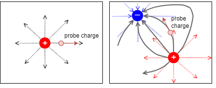
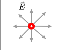
Take a charge ($+1nC$) and position it. \ Measure the field across a sample charge (a sensor).
The simulation in figure 2 was already briefly considered in the first chapter. Here, however, another point is to be dealt with.
In the simulation, please position a negative charge $Q$ in the middle and deactivate electric field. The latter is done via the hook on the right. Now the situation is close to reality, because a charge shows no effect at first sight.
For impact analysis, a sample charge $q$ is placed in the vicinity of the existing charge $Q$ (in the simulation, the sample charge is called “sensors”). It is observed that the charge $Q$ causes a force on the sample charge. This force can be determined at any point in space with magnitude and direction. It acts in space in a similar way to gravity. The description of the state in space changed by the charge $Q$ is described with the help of a field.
The concept of the field shall now be briefly considered in a little more detail.
- The introduction of the field separates the cause from the effect.
- The charge $Q$ causes the field in space.
- The charge $q$ in space feels a force as an effect of the field.
- This distinction becomes important again in this chapter.
Also in electrodynamics this distinction becomes clear: the field there corresponds to photons, i.e. to a transmission of effects with the finite (light)speed $c$.
- As with physical quantities, there are different-dimensional fields:
- In a scalar field, a single number is assigned to each point in space.
E.g.- temperature field $T(\vec{x})$ on the weather map or in an object
- pressure field $p(\vec{x})$
- In a vector field, each point in space is assigned several numbers in the form of a vector. This reflects the action along the spatial coordinates.
For example.- gravitational field $\vec{g}(\vec{x})$ pointing to the center of mass of the object.
- electric field $\vec{E}(\vec{x})$
- magnetic field $\vec{H}(\vec{x})$
- If each point in space is associated with a two- or more-dimensional physical quantity - that is, a tensor - then this field is called a tensor field. Tensor fields are relevant in mechanics (e.g., stress tensor) but are not necessary for electrical engineering.
Vector fields can be stated as:
- Effects along spatial axes $x$,$y$ and $z$ (Cartesian coordinate system).
- Effect in magnitude and direction vector (polar coordinate system)
Remember:
- Fields describe a physical state of space.
- Here, a physical quantity is assigned to each point in space.
- The electrostatic field is described by a vector field.
The electric field
Thus, to determine the electric field, a measure of the strength of the field is now needed. From the first chapter the Coulomb-force between two charges $Q_1$ and $Q_2$ is known:
\begin{align*} F_C = {{{1} \over {4\pi\cdot\varepsilon}} \cdot {{Q_1 \cdot Q_2} \over {r^2}}} \end{align*}
In order to obtain a measure of the strength of the electric field, the force on a (fictitious) sample charge $q$ is now considered.
\begin{align*} F_C &= {{{1} \over {4\pi\cdot\varepsilon}} \cdot {{Q_1 \cdot q} \over {r^2}}} \\ &= \underbrace{{{1} \over {4\pi\cdot\varepsilon}} \cdot {{Q_1} \over {r^2}}}_\text{=independent of q} \cdot q \\ \end{align*}
The left part is therefore a measure of the strength of the field, i.e. independent of the size of the sample charge $q$. The strength of the electric field is thus given by
$E = {{1} \over {4\pi\cdot\varepsilon}} \cdot {{Q_1} \over {r^2}} \quad$ with $[E]={{[F]}\over{[q]}}=1 {{N}\over{As}}=1 {{N\cdot m}\over{As \cdot m}} = 1 {{V \cdot A \cdot s}\over{As \cdot m}} = 1 {{V}\over{m}}$
The result is therefore \begin{align*} \boxed{F_C = E \cdot q} \end{align*}
Notice:
- The procharge $q$ is always considered to be ppositive. It is used only as a thought experiment and has no repercussion on the sampled charge $Q$.
- The sampled charge is a point charge.
Notice:
A charge $Q$ generates at a measuring point $P$ an electric field strength $\vec{E}(Q)$, which is given by- the magnitude $|E|=\Bigl| {{1} \over {4\pi\cdot\varepsilon}} \cdot {{Q_1} \over {r^2}} \Bigl| $ and
- the direction of the force $\vec{F_C}$ on a sample charge at rest at the measurement point $P$. This is given by the unit vector $\vec{e_r}={{\vec{F_C}}\over{|F_C|}}$ in that direction.
The direction of the electric field is switchable in figure 2 via the “Electric Field” option on the right.
The electric field can also be viewed again in this video.
Electric field lines
Fig. 4: examples of field lines
Superposition of fields
(CC-BY-SA 4.0: MINT bridge course)
Electric field lines result as the (fictitious) path of a sample charge. Thus also electric field lines of several charges can be determined. However, these also result from a superposition of the individual effects - i.e. field strengths - at a measuring point $P$.
The superposition is sketched in figure 4 and can be viewed again in the simulation in figure ##. In addition, this is described again in more detail in the video on the right.
Merke:
- The electrostatic field is a source field. This means there are sources and sinks.
This is equal to: The electric field lines have a beginning (at a positive charge) and an end (at a negative charge). - From the field line diagrams, the following can be obtained:
- Direction of the field ($\hat{=}$ tangent to the field line).
- Magnitude of the field ($\hat{=}$ number of field lines per unit area).
- The magnitude of the field strength along a field line is usually not constant.
Tasks
Task 5.1.1 Electric field example tasks
Task 5.1.2 Field lines
.
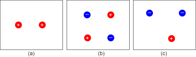
Sketch the field line plot for the charge configurations given in figure 6.
Notice:
- It is the overlaid image that is sought.
- Make sure that it is a source field.
5.2 Electric charge and Coulomb force (reloaded)
Goals
After this lesson, you should:
- Be able to determine the direction of the forces using given charges.
- be able to represent the acting force vectors in a sketch.
- be able to determine a force vector by superimposing several force vectors using vector calculus.
- be able to state the following quantities for a force vector:
- Force vector in coordinate representation
- magnitude of the force vector
- Angle of the force vector
The electric charge and Coulomb force has already been described in chapter 1. However, some points are to be caught up here to it.
Direction of the Coulomb force and superposition
Fig. 7: direction of coulomb force
.
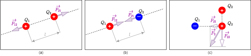
In the case of the force, the direction has been considered so far, e.g. direction towards the sample charge, but for future explanations it is important to include the cause-effect in the naming. In figure 7 (a) and (b) the convention is shown again: A force $\vec{F}_{21}$ acts on charge $Q_2$ and is caused by charge $Q_1$. As a mnemonic you can remember “tip-foot” (first the effect, then the cause).
Furthermore, several forces on a charge can be superimposed to a resulting force. Strictly speaking, it must hold that $\varepsilon$ is constant in the structure. For example, the resultant force in figure 7 Fig. (c) on $Q_3$ becomes equal to: $\vec{F_3}= \vec{F_{31}}+\vec{F_{32}}$.
Geometric Distribution of Charges
In previous chapters only single charges (e.g. $Q_1$, $Q_2$) were considered.
- The charge $Q$ was previously reduced to a point charge.
This can be used, for example, for the elementary charge or for extended charged objects from a large distance. The distance is sufficiently large if the ratio between the largest object extent and the distance to the measurement point $P$ is small.
- If the charges are lined up along a line, this is called a line charge.
Examples of this are a straight trace on a circuit board or a piece of wire. Furthermore, this also applies to an extended charged object, which has exactly an extension that is no longer small in relation to the distance. For this purpose, the charge $Q$ is considered to be distributed over the line. Thus, a (line) charge density $\rho_l$ can be determined:$\rho_l = {{Q}\over{l}}$
or, in the case of different charge densities on subsections:
$\rho_l = {{\Delta Q}\over{\Delta l}} \rightarrow \rho_l(l)={{d}\over{dl}} Q(l)$
- A area charge is spoken of when the charge is to be regarded as distributed over an area. \ Examples of this are the floor or a plate of a capacitor. Again, an extended charged object can be considered if there are two extensions which are no longer small in relation to the distance (e.g. surface of the earth). Again, a (surface) charge density $\rho_A$ can be determined:
$\rho_A = {{Q}\over{A}}$
or if there are different charge densities on partial surfaces:
$\rho_A = {{\Delta Q}\over{\Delta A}} \rightarrow \rho_A(A) ={{d}\over{dA}} Q(A)={{d}\over{dx}}{{d}\over{dy}} Q(A)$
- Finally, a space charge is the term for charges that span a volume. \here examples are plasmas or charges in extended objects (e.g. in semiconductor). as with the other charge distributions, a (space) charge density $\rho_V$ can be calculated here:
$\rho_V = {{Q}\over{V}}$
or for different charge density in partial volumes:
$\rho_V = {{\Delta Q}\over{\Delta V}} \rightarrow \rho_V(V) ={{d}\over{dV}} Q(V)={{d}\over{dx}}{{d}\over{dy}}{{d}\over{dz}} Q(V)$
Types of fields depending on the charge distribution
There are two different types of fields:
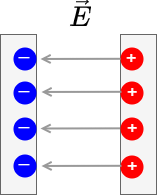
In homogeneous fields, magnitude and direction are constant throughout the field range. This field form is idealized to exist within plate capacitors. e.g., in the plate capacitor (figure 9), or in the vicinity of widely extended bodies.
For inhomogeneous fields, the magnitude and/or direction of the field strength changes from place to place. This is the rule in real systems, even the field of a point charge is inhomogeneous (figure 10).
Tasks
5.3 Work and Potential
Goals
After this lesson, you should:
- know how work is defined in the electrostatic field.
- be able to describe when work occurs and when it does not when a charge is moving.
- know the definition of electric voltage and be able to calculate it in an electric field.
- understand why the calculation of voltage is independent of displacement.
- know what a potential difference is and recognise or be able to state equipotential surfaces (lines).
- be able to determine a potential curve for a given arrangement.
A detailed explanation can be found in the KIT bridge course. It is recommended to work through this independently.
In particular, this applies to:
- Chapter “4.1.2 electric field” from video 221 to the end of the tasks.
- Chapter “4.1.3 work, potential, voltage” to the end of the tasks and the Additional Content
Energy required to displace a charge in the field
Fig. 11: Observation of work in a homogeneous electric field
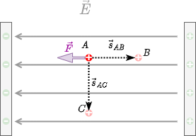
First, the situation of a charge in a homogeneous electric field shall be considered. As we have seen so far, the magnitude of E is constant and the field lines are parallel. Now a positive charge $q$ is to be brought into this field.
If this charge would be free movable (e.g. electron in vacuum or in extended conductor) it would be accelerated along field lines. Thus its kinetic energy increases. Because the whole system of plates (for field generation) and charge however does not change its energetic state - thermodynamically the system is closed. From this follows: if the kinetic energy increases, the potential energy must decrease.
From mechanics is known, here done work (thus energy done by forces) is defined by force along a way.
In a homogeneous field, the following holds for a force action producing motion along a field line from $A$ to $B$ (see figure 11):
\begin{align*}
W_{AB} = F_C \cdot s
\end{align*}
For a motion parallel to a field line (i.e. from $A$ to $C$) $W_{AC}=0$ results. This situation is similar to the movement of a weight in the gravitational field at the same height. There, too, no energy is released or absorbed. For any direction through the field the part of the path has to be considered, which is parallel to the field lines. This results from the angle $\alpha$ between $\vec{F}$ and $\vec{s}$: \begin{align*} W_{AB} = F_C \cdot s \cdot cos(\alpha) = \vec{F_C}\cdot \vec{s} \end{align*}
The work $W_{AB}$ here describes the energy difference experienced by the charge $q$.
Similar to the electric field, we now look for a quantity that is independent of the (sample) charge $q$ in order to describe the energy component. This is done by the potential $\varphi$ (also potential). The potential in a homogeneous field is defined as:
\begin{align} \varphi_{AB} = {{W_{AB}}\over{q}} = {{F_C \cdot s}\over{q}} = {{E \cdot q \cdot s}\over{q}} = E \cdot s_{AB} \end{align}
Notice:
The potential $\varphi$ in an $E$-field is the ability to do work $W$.To obtain a general approach to inhomogeneous fields and arbitrary paths $s_{AB}$, it helps (as is so often the case) to decompose the problem into small parts. In the concrete case, these are small path segments on which the field can be assumed to be homogeneous. These are to be assumed to be infinitesimally small in the extreme case (i.e., from $s$ to $\delta s$ to $ds$):
\begin{align} W_{AB} = \vec{F_C}\cdot \vec{s} \quad \rightarrow \quad \Delta W = \vec{F_C}\cdot \Delta \vec{s}\quad \rightarrow \quad dW = \vec{F_C}\cdot d \vec{s} \end{align}
The total energy now results from the sum or integration of these path sections:
\begin{align*} W_{AB} &= \int_{W_A}^{W_B} dW \ &= \int_{A}^{B} \vec{F_C}\cdot d \vec{s} \\ &= \int_{A}^{B} q \cdot \vec{E} \cdot d \vec{s} \\ &= q \cdot \int_{A}^{B} \vec{E} \cdot d \vec{s} \end{align*}
The potential is therewith:
\begin{align*} \varphi_{AB} &= {{W_{AB}}\over{q}} &= \int_{A}^{B} \vec{E} \cdot d \vec{s} \end{align*}
The potential difference $\varphi_{AB}$ is also called voltage $U_{AB}$. The voltage is measured in volts.
It is interesting that it does not matter which way the integration takes place. So it doesn't matter how the charge gets from $A$ to $B$, the energy or potential difference is always the same. This follows from the fact that a charge $q$ at a point $A$ in the field has a unique potential energy. No matter how this charge is moved to a point $B$ and back again: as soon as it gets back to the point $A$, it has the same energy again. So the potential difference of the way there and back must be equal in magnitude.
This concept has already been applied as a mesh theorem in circuits (see chapter 2). However, it is also valid in other structures and arbitrary electrostatic fields.
\begin{align*} \varphi_{AB} &= \int_{A}^{B} \vec{E} \cdot d \vec{s} \quad && | \vec{E} \text{ and } d\vec{s} \text{ run parallel } \\ \varphi_{AB} &= \int_{A}^{B} E \cdot ds \quad && | \text{E=const.} \\ \varphi &= E \cdot \int_{0}^{d} ds \quad && | s \text{ starts counting at the negative plate. } d \text{ denotes the distance between the two plates }\\ \varphi &= E \cdot d \quad && | \varphi_{AB} \text{ ecorresponds to the voltage applied to the capacitor } U \\ U &= E \cdot d \end{align*}
Merke:
Returning to the starting point from any point $A$ after a closed circuit, the circuit voltage along the closed path is 0. A closed path is mathematically expressed as a ring integral:\begin{align} \varphi = \oint \vec{E} \cdot d \vec{s} = 0 \end{align}
Or spoken differently: In the electrostatic field there are no self-contained field lines.
A field $\vec{X}$ which satisfies the condition $\oint \vec{X} \cdot d \vec{s}=0$ is called vortex-free or potential field.
From the potential difference, or the voltage, the work in the electrostatic field results with:
\begin{align*} \boxed{W_{AB}= q \cdot U_{AB}} \end{align*}
Equipotential lines

If a charge $q$ becomes perpendicular to the field lines, it experiences neither energy gain nor loss. The voltage along this path is $0V$. All points between which the voltage of $0V$ is applied are at the same potential level. The connection of these points is called:
- equipotential lines for a 2-dimensional representation of the field.
- equipotential surfaces for a 3-dimensional field
This corresponds in the gravity field to a movement on the same contour line. The contour lines are often drawn in (hiking) maps, cf. figure 13. If one moves along the contour lines, no work is done.
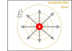
The equipotential surfaces are usually drawn with a fixed step size, e.g. $1V$, $2V$, $3V$, … . Since the electric field is higher near charges, equipotential surfaces are also closer together there. In figure 14, the equipotential surfaces of a point charge are shown.
Fig. 14: Field lines and equipotential surfaces of a point charge
.
Reference potential
5.4 Conductors in the electrostatic field
Goals
After this lesson, you should:
- know that no current flows in a conductor in an electrostatic field.
- know how charges in a conductor are distributed in the electrostatic field.
- Be able to sketch the field lines at the surface of the conductor.
- Understand the effect of the influence of an external electric field.
Up to now, charges were considered which were either rigid or freely movable. At the following, charges at an electric conductor are to look at. These are only free movable within the conductor. At first an ideal conductor without resistance is considered.
Stationary state of charges without external field
Fig. 18: Viewing a charged metal ball
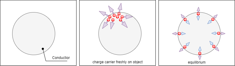
In the first thought experiment, a conductor (e.g. a metal plate) is charged, see figure 18. The additional charges create an electric field. Thus, a resultant force acts on each charge. The cause of this force is the fields of the surrounding electric charges. So the charges repel and move apart.
The movement of the charge continues until a force equilibrium is reached. In this steady state, there is no longer a resultant force acting on the single charge. In figure 18 this can be seen on the right: the repulsive forces of the charges are counteracted by the attractive forces of the atomic shells.
Results:
- The charge carriers are distributed on the surface.
- Due to the dispersion of the charges, the interior of the conductor is free of fields.
- All field lines are perpendicular to the surface. Because: if they were not, there would be a tangential component of the field, i.e. along the surface. Thus a force would act on charge carriers and they would move accordingly.
Influenza
Fig. 21: Viewing the influential charge separation
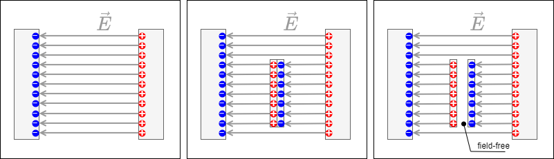
In the second thought experiment, an uncharged conductor (e.g. a metal plate) is brought into an electrostatic field (figure 21). The external field or the resulting Coulomb force causes the moving charge carriers to be displaced.
Results:
- The charge carriers are still distributed on the surface.
- Now an equilibrium is reached, when just so many charges have moved, that the field strength inside the conductor disappears (again).
- The field lines leave the surface again at right angles. Again, a tangential component would cause a charge shift in the metal.
This effect of charge displacement in conductive objects by an electrostatic field is called influence. Influence charges can be separated (figure 21 right). If we look at the separated influence charges without the external field, their field is again just as strong in magnitude as the external field only opposite.
Merke:
- The seat of an influenced charge is always the conductor surface. This results in a surface charge density $\varrho_A = {{\Delta Q}\over{\Delta A}}$
- The conductor surface in the electrostatic field is always an equipotential surface. Thus, the field lines always originate and terminate perpendicularly on conductor surfaces.
- The interior of the conductor is always field-free (Faraday effect: metallic enclosures shield electric fields).
How can the conductor surface be an equipotential surface despite different charge on both sides? Equipotential surfaces are defined only by the fact that the movement of a charge along such a surface does not require/produce a change in energy. Since the interior of the conductor is field free, movement there can occur without a change in energy. As the potential between two points is independent of the path between them, a path along the surface is also possible without energy expenditure.
Tasks
Application of Influence: Protective bag against electrostatic charge / discharge (cf. Video)
Task 5.4.1 Simulation
In the simulation program of Falstad the courses of equipotential surfaces and electric field strength at different objects can be represented.
- Open the simulation program via the link
- Select: “Setup: cylinder in field”, “Floor: equipotentials” and “Display: Field Vectors”.
- The field of an infinitely long cylinder in a homogeneous electric field is now displayed in section. The solid lines show the equipotential surfaces. The small arrows show the electric field strength.
- What can be said about the potential distribution on the cylinder?
- On the left half the field lines enter the body, on the right half they leave the body. What can be said about the charge carrier distribution at the surface? Check also the representation “Color: charge”!
- Is there an electric field inside the body? Check also the diagram “Floor: Field lines”!
- Is this cylinder metallic, semiconducting or insulating?
5.5 The electric displacement flux and Gaussian theorem of electrostatics
The electric displacement (flux) density
Goals
After this lesson, you should:
- know how to get the electric displacement flux from single charges
- be able to state for a given area the displacement flux density of an arrangement
- know the general meaning of Gauss' theorem of electrostatics
- be able to choose a closed enveloping surface appropriately and apply Gauss' theorem
Fig. 26: Influenced charge separation and displacement flow

Now we want to consider the situation at the two conductive plates with the area $\Delta A$ in the electrostatic field $\vec{E}$ in vacuum a little more exactly. For this purpose, the plates shall first be brought into the field separately. As written in figure 26 on the left, the influence in a single plate is not considered. Rather, we are now interested in what happens when the plates are brought together. In this case, graphically speaking, just for each field line ending on the pair of plates, a single charge must move from one plate to the other. This ability to separate charges (i.e. to generate influence) is another ability of space.
In the previous arrangement (homogeneous field, all surfaces parallel to each other), the surface charge density $\varrho_A = {{\Delta Q}\over{\Delta A}}$ thus influenced is proportional to the external field $E$. It holds:
\begin{align*} \varrho_A = {{\Delta Q}\over{\Delta A}} \sim E \\ \varrho_A = {{\Delta Q}\over{\Delta A}} = \varepsilon \cdot E \end{align*}
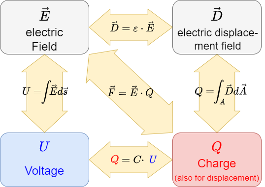
The displacement (flux) density is now defined as.
\begin{align} \boxed{\vec{D} = \varepsilon \cdot \vec{E}} \end{align}
The displacement (flux) density has the unit “charge per area”, i.e. $As/m^2$. The displacement (flux) density is also a field. It points in the same direction as the electrostatic field $\vec{E}$.
Why is now a second field introduced? This shall become clearer in the following, but first it shall be considered again how the electrostatic field $\vec{E}$ was defined. This resulted from the Coulomb force, i.e. the action on a sample charge. The displacement density, on the other hand, is not described by an action, but caused by charges. The two are related by the above equation. It will be shown in later sub-chapters that the different influences from the same cause of the field can produce different effects on other charges.
The permittivity (or dielectric conductivity) $\varepsilon$ thus results as a constant of proportionality between $D$-field and $E$-field. The inverse ${{1}\over{\varepsilon}}$ is a measure of how much effect ($E$-field) is available from the cause ($D$-field) at a point. In vacuum, $\varepsilon= \varepsilon_0$, the electric field constant.
General relationship between charge Q and displacement density D
Up to now, only a homogeneous field and an observation surface perpendicular to the field lines were considered. Thus only equipotential surfaces (e.g. a metal foil) were considered. In that case it was found that the charge is equal to the displacement density on the surface: $\Delta Q = D\cdot \Delta A$.
This formula is now to be extended to arbitrary surfaces and inhomogeneous fields. As with the potential and other physical problems, the problem is to be broken down into smaller subproblems, solved and then summed up. For this purpose a small area element $\Delta A = \Delta x \cdot \Delta y$ is needed. In addition, the position of the area in space should be taken into account. This is possible if the cross product is chosen: $\Delta \vec{A} = \Delta \vec{x} \cdot \Delta \vec{y}$, since so is the surface normal. In what follows, the cross product will be relevant to the calculation, but the consequences of the cross product will be:
- The magnitude of $\Delta \vec{A}$ is equal to the area $\Delta A$.
- The direction of $\Delta \vec{A}$ is perpendicular to the area.
In addition, let $\Delta A$ now become infinitesimally small, that is, $dA = dx \cdot dy$.
1. problem: inhomogeneity → solution: shrink area
First, we shall still assume an observation surface perpendicular to the field lines, but an inhomogeneous field. In the inhomogeneous field, the magnitude of $D$ is no longer constant. In order to correct this, $dA$ is chosen so small that just “only one field line” passes through the surface. In this case D is homogeneous again. Thus holds:
$Q = D\cdot A$
\begin{align*} Q = D\cdot A \quad \rightarrow \quad dQ = D\cdot dA \end{align*}
2nd problem: arbitrary surface → solution: vectors
Now assume an arbitrary surface. Thus the $\vec{D}$-field no longer penetrates through the surface at right angles. But for the influence only the rectangular part was relevant. So only this part has to be considered. This results from consideration of the cosine of the angle between (right-angled) surface normal and $\vec{D}$-field:
\begin{align*} dQ = D\cdot dA \quad \rightarrow \quad dQ = D\cdot dA \cdot cos(\alpha) = \vec{D} \cdot d \vec{A} \end{align*}
3. summing up
Since so far only infinitesimally small surface pieces were considered must now be integrated again to a total surface. If a closed enveloping surface around a body is chosen, the result is:
\begin{align} \boxed{\int dQ = \iint_{\text{hull}} \vec{D} \cdot d \vec{A} = Q} \end{align}
The “sum” of the $D$-field emanating over the surface is thus just as large as the sum of the charges contained therein, since the charges are just the sources of this field. This can be compared vividly with a bordered swamp area with water sources and sinks:
- The sources in the marsh correspond to the positive charges, the sinks to the negative charges. The formed water corresponds to the $D$-field.
- The sum of all sources and sinks equals in this case just the water stepping over the edge.
Applications
Are calculated in the course.
Spherical capacitor
Spherical capacitors are now rarely found in practical applications. In the Van-de-Graaff generator, spherical capacitors are used to store the high DC voltages. The earth also represents a spherical capacitor. In this context, the electric field strength of $100...300 V/m$ in the atmosphere is remarkable, since several hundred volts would have to be present between head and foot (for resolution, see the article Spannung lieg in der Luft in Bild der Wissenschaft).
Plate capacitor
The relation between the $E$-field and the voltage $U$ on the ideal plate capacitor is to be derived from the integral of the displacement density $\vec{D}$: \begin{align*} Q = \iint_{\text{shell}} \vec{D} \cdot d \vec{A} \end{align*}
Outlook
The consideration of the displacement-flux-density also solved a problem, which arose quite for at electric circuits: From considerations about magnetic fields the following quite obvious sounding fact can be led: In a series-connected, switched circuit, the current at each point is the same. But if this series circuit contains a capacitor, no electric current can flow inside! The solution is to understand a temporal change of the displacement flux also as a current, which can be generated a magnetic field (thus vortex). Mathematically, vortices are described via the Curl (in German: Rotation) - a multidimensional differential operator. A deeper derivation and solution is not considered in the first semester. However, the application will show that the above equation plays a central role in electrical engineering. It is part of the so-called Maxwell's equations.
5.6 Non-conductor in electrostatic field
Goals
After this lesson, you should:
- know the two field-describing quantities of the electrostatic field
- be able to describe and apply the relationship between these two quantities via the material law
- understand the effect of an electrostatic field on an insulator
- know what the effect of dielectric polarisation does
- be able to relate the term dielectric strength to a property of insulators and know what it means
material-law-of-electrostatics
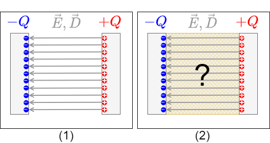
First of all, a thought experiment is to be carried out again (see figure 31):
- First a charged plate capacitor in vacuum is assumed, which is separated from the voltage source after charging.
- Next, the intermediate region is to be filled with a material.
Think about how $E$ and $D$ would change before you unfold the subsection.
Why might which of the two quantities change?
- The material law of electrostatics
-
You may have considered what happens to the charge $Q$ on the plates. This charge cannot leave the plates. So $Q = \iint_{\text{envelope}} \vec{D} \cdot d \vec{A}$ cannot change.
Since the sheath as a fictitious surface around an electrode does not change either, $\vec{D}$ cannot change either.On the other hand, polarizable materials in the capacitor can align themselves. This dampens the effective field. Maybe you remember what the “acting field” was: the $E$-field. So the $E$-field becomes smaller (see figure 32).
Previously:
\begin{align*} D = \varepsilon_0 \cdot E \end{align*}
The determined change is packed into the material constant $\varepsilon_r$. This gives the material law of electrostatics:
\begin{align*} \boxed{D = \varepsilon_r \cdot \varepsilon_0 \cdot E} \end{align*}
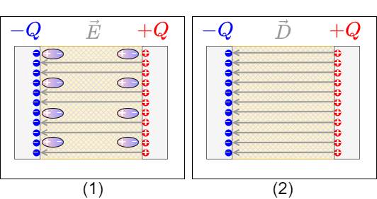
Since the charge $Q$ cannot vanish from the capacitor in this experimental setup and thus $D$ remains constant, the $E$ field must become smaller for $\varepsilon_r>1$.
figure 32 is drawn here in a simplified way: the alignable molecules are evenly distributed over the material and are thus also evenly aligned. Accordingly, the E-field is uniformly attenuated.
Remember:
- The material constant $\varepsilon_r$ is called relative permittivity, relative permittivity, or dielectric constant.
- Relative permittivity is unitless and indicates how much the electric field strength decreases with the presence of material for the same charge.
- The relative permittivity $\varepsilon_r$ is always greater than or equal to 1 for dielectrics (i.e., nonconductors).
- The relative permittivity depends on the polarizability of the material, i.e. the possibility to align the molecules in the field. Correspondingly, relative permittivity depends on frequency and often direction and temperature.
Outlook
If now the relative permittivity $\varepsilon_r$ depends on the possibility to align the molecules in the field, the following interesting relation arises: if frequencies are “caught”, at which the oscillation of the molecule can build up, the energy of the external field is absorbed by the molecule. This build-up is similar to the shattering of a wine glass at a suitable irradiated frequency and is called resonance. Materials can be analysed on the basis of the resonance frequencies. These resonance frequencies are enormously high (1 GHz to 1'000'000 GHz) and in these frequencies the $E$-field detaches from the conductor. This may sound strange, but it becomes a bit more illustrative in the 2nd semester with the resonant circuit. For the 1st semester it is more than sufficient that in the range of 1'000'000 GHz is the visual light, which is obviously not bound to a conductor. But this also makes clear that the relative permittivity $\varepsilon_r$ for high frequencies also has to do with the absorption (and reflection) of electromagnetic waves.Some values of the relative permittivity $\varepsilon_r$ for dielectrics are given in table 1.
Dielectric strength of dielectrics
- The dielectrics act as insulators. The flow of current is therefore prevented
- The ability to insulate is dependent on the material.
- If a maximum field strength $E_0$ is exceeded, the insulating ability is eliminated
- One says: The insulator breaks down. This means that above this field strength a current can flow through the insulator.
- Examples are: Lightning in a thunderstorm, ignition spark, glow lamp in a phase tester
- The maximum field strength $E_0$ is called dielectric strength.
- $E_0$ depends on the material (see table 2), but also on other factors (temperature, humidity, …).
tasks
Task 5.6.1 Thought Experiment
Consider what would have happened if the plates had not been detached from the voltage source in the above thought experiment (figure 31).
5.7 Capacitors
Goals
After this lesson, you should:
- know what a capacitor is and how capacitance is defined
- know the basic equations for calculating a capacitor and be able to apply them
- be able to imagine a plate capacitor and know examples of its use You also have an idea of what a cylindrical or spherical capacitor looks like and what examples of its use there are
- know the characteristics of the E-field, D-field and electric potential in the three types of capacitors presented here
Capacity
- A capacitor is defined by the fact that there are two electrodes (= conductive areas), which are separated by a dielectric (= non-conductor).
- This makes it possible to build up an electric field in the capacitor without charge carriers moving through the dielectric.
- The characteristic of the capacitor is the capacity $C$.
- In addition to the capacitance, every capacitor also has a resistance and an inductance. However, both of these are usually very small.
- Examples are
- the electrical component “capacitor”,
- an open switch,
- a wire to ground,
- a human being
$\rightarrow$ Thus, for any arrangement of two conductors separated by an insulating material, a capacitance can be specified.
The capacity $C$ can be derived as follows:
- It is known that $U = \int \vec{E} d \vec{s} = E \cdot l$ and hence $E= {{U}\over{l}}$ or $D= \varepsilon_0 \cdot \varepsilon_r \cdot {{U}\over{l}}$.
- Furthermore, $\iint_{\text{envelope}} \vec{D} \cdot d \vec{A} = Q$ by the idealized form of the plate capacitor: $Q=D \cdot A$.
- Thus, the charge $Q$ is given by: \begin{align*} Q = \varepsilon_0 \cdot \varepsilon_r \cdot {{U}\over{l}} \cdot A \end{align*}
- This means that $Q \sim U$, given the geometry (i.e., $A$ and $d$) and the dielectric ($\varepsilon_r $).
- So it is reasonable to determine a proportionality factor ${{Q}\over{U}}$.
The capacitance $C$ of an idealized plate capacitor is defined as
\begin{align*} \boxed{C = \varepsilon_0 \cdot \varepsilon_r \cdot {{A}\over{l}} = {{Q}\over{U}}} \end{align*}
This relationship can be examined in more detail in the following simulation:
- capacitor lab
-
If the simulation is not displayed optimally, this link can be used.
Designs and types of capacitors
To calculate the capacitances of different designs, the definition equations of $\vec{D}$ and $\vec{E}$ are used. This can be viewed in detail e.g. in this video.
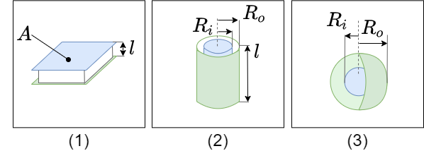
Based on the geometry, different equations result (see also figure 34).
| Shape of the capacitor | Parameter | Equation for the capacitance | |
|---|---|---|---|
| plate capacitor | area $A$ of plate distance $l$ between plates | \begin{align*}C = \varepsilon_0 \cdot \varepsilon_r \cdot {{A}\over{l}} \end{align*} | |
| cylinder capacitor | radius of outer conductor $R_a$ radius of inner conductor $R_i$ length $l$ | \begin{align*}C = \varepsilon_0 \cdot \varepsilon_r \cdot 2\pi {{l}\over{ln \left({{R_a}\over{R_i}}\right)}} \end{align*} | |
| spherical capacitor | radius of outer spherical conductor $R_a$ radius of inner spherical conductor $R_i$ | \begin{align*}C = \varepsilon_0 \cdot \varepsilon_r \cdot 4 \pi {{R_i \cdot R_a}\over{R_a - R_i}} \end{align*} |
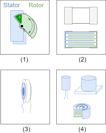
In figure 35 different designs of capacitors can be seen:
- rotary variable capacitor (also variable capacitor or trim capacitor).
- A variable capacitor consists of two sets of plates: a fixed set and a movable set (stator and rotor). These represent the two electrodes.
- The movable set can be rotated radially into the fixed set. This covers a certain area $A$.
- The size of the area is increased by the number of plates. Nevertheless, only small capacities are possible because of the necessary distance.
- Air is usually used as the dielectric, occasionally small plastic or ceramic plates are used to increase the dielectric constant.
-
- In the multilayer capacitor, there are again two electrodes. Here, too, the area $A$ (and thus the capacitance $C$) is multiplied by the finger-shaped interlocking.
- Ceramic is used here as the dielectric.
- The multilayer ceramic capacitor is also called KerKo or MLCC.
- The variant shown in (2) is an SMD variant (surface mound device).
- Disk capacitor
- A ceramic is also used as dielectric for the disk capacitor. This is positioned as a round disc between two electrodes.
- Disc capacitors are designed for higher voltages, but have a low capacitance (in the microfarad range).
- Electrolytic capacitor, in German also called Elko for Elektrolytkondensator
- In electrolytic capacitors, the dielectric is an oxide layer formed on the metallic electrode. the second electrode is the liquid or solid electrolyte.
- Different metals can be used as the oxidized electrode, e.g. aluminium, tantalum or niobium.
- Because the oxide layer is very thin, a very high capacity results (depending on the size: up to a few millifarads).
- Important for the application is that it is a polarized capacitor. I.e. it may only be operated in one direction with DC voltage. Otherwise, a current can flow through the capacitor, which destroys it and is usually accompanied by an explosive expansion of the electrolyte. To avoid reverse polarity, the negative pole is marked with a dash.
- The electrolytic capacitor is built up wound and often has a cross-shaped predetermined breaking point at the top for gas leakage.
- film capacitor, in German also called Folko, for Folienkondensator.
- A material similar to a “chip bag” is used as an insulator: a plastic film with a thin, metallized layer.
- The construction shows a high pulse load capacity and low internal ohmic losses.
- In the event of electrical breakdown, the foil enables “self-healing”: the metal coating evaporates locally around the breakdown. Thus the short-circuit is cancelled again
- With some manufacturers this type is called MKS (Mmetallized foilccapacitor, Polyester).
- Supercapacitor (engl. Super-Caps)
- As a dielectric is - similar to the electrolytic capacitor - very thin. In the actual sense, there is no dielectric at all.
- The charges are not only stored in the electrode, but - similar to a battery - the charges are transferred into the electrolyte. Due to the polarization of the charges, they surround themselves with a thin (atomic) electrolyte layer. The charges then accumulate at the other electrode.
- Supercapacitors can achieve very large capacitance values (up to the kilofarad range), but only have a low maximum voltage


In figure 34 are shown different capacitors:
- Above two SMD capacitors
- On the left a $100\mu F$ electrolytic capacitor
- On the right a $100nF$ MLCC in the commonly used Surface-mount_technology 0603 (1.6mm x 0.8mm)
- below different THT capacitors (Through Hole Technology)
- a big electrolytic capacitor with $10mF$ in blue, the positive terminal is marked with $+$
- in the second row is a Kerko with $33pF$ and two Folkos with $1,5\mu F$ each
- in the bottom row you can see a trim capacitor with about $30pF$ and a tantalum electrolytic capacitor and another electrolytic capacitor
Various conventions]] have been established for designating the capacitance value of a capacitor various conventions.
Electrolytic capacitors can explode!
Notice:
- There are polarized capacitors. With these, the installation direction and current flow must be observed, as otherwise an explosion can occur.
- Depending on the application - and the required size, dielectric strength and capacitance - different types of capacitors are used.
- The calculation of the capacitance is usually not via $C = \varepsilon_0 \cdot \varepsilon_r \cdot {{A}\over{l}} $ . The capacitance value is given.
- The capacitance value often varies by more than $\pm 10\%$. I.e. a calculation accurate to several decimal places is rarely necessary/possible.
- The charge current seems to be able to flow through the capacitor because the charges added to one side induce correspondingly opposite charges on the other side.
5.8 Interconnection of capacities
Goals
After this lesson, you should:
- be able to recognise a series connection of capacitors and distinguish it from a parallel connection
- be able to calculate the resulting total capacitance of a series or parallel circuit
- know how the total charge is distributed among the individual capacitors in a parallel circuit
- be able to determine the voltage across a single capacitor in a series circuit
Capacitor series connection
If capacitors are connected in series, the charging current $I$ into the individual capacitors $C_1 ... C_n$ is equal. Thus, the charges absorbed $\delta Q$ are also equal: \begin{align*} \Delta Q = \Delta Q_1 = \Delta Q_2 = ... = \Delta Q_n \end{align*}
Furthermore, after charging, a voltage is formed across the series circuit which corresponds to the source voltage $U_q$. This results from the addition of the partial voltages across the individual capacitors. \begin{align*} U_q = U_1 + U_2 + ... + U_n = \sum_{k=1}^n U_k \end{align*}
It holds for the voltage $U_k = \Large{{Q_k}\over{C_k}}$.
If all capacitors are initially discharged, then $U_k = \Large{{\Delta Q}\over{C_k}}$ holds.
Thus
\begin{align*}
U_q &= &U_1 &+ &U_2 &+ &... &+ &U_n &= \sum_{k=1}^n U_k \\
U_q &= &{{\Delta Q}\over{C_1}} &+ &{{\Delta Q}\over{C_2}} &+ &... &+ &{{\Delta Q}\over{C_3}} &= \sum_{k=1}^n {{1}\over{C_k}}\cdot \Delta Q \\
{{1}\over{C_{ges}}}\cdot \Delta Q &= &&&&&&&&\sum_{k=1}^n {{1}\over{C_k}}\cdot \Delta Q
\end{align*}
Thus, for the series connection of capacitors $C_1 ... C_n$ :
\begin{align*} \boxed{ {{1}\over{C_{ges}}} = \sum_{k=1}^n {{1}\over{C_k}} } \end{align*} \begin{align*} \boxed{ \Delta Q_k = const.} \end{align*}
For initially uncharged capacitors, (voltage divider for capacitors) holds: \begin{align*} \boxed{Q = Q_k} \end{align*} \begin{align*} \boxed{U_{ges} \cdot C_{ges} = U_{k} \cdot C_{k} } \end{align*}
In the simulation on the right, besides the parallel connected capacitors $C_1$, $C_2$,$C_3$, an ideal voltage source $U_q$, a resistor $R$, a switch $S$ and a lamp are installed.
- The switch $S$ allows the voltage source to charge the capacitors.
- The resistor $R$ is necessary because the simulation cannot represent instantaneous charging. The resistor limits the charging current to a maximum value.
Further details about the resistor are described in the chapter Switching operations on RC combinations. - The capacitors can be discharged again via the lamp.
This derivation is also well explained, for example, in this video.
parallel-circuit-capacitors
If capacitors are connected in parallel, the voltage $U$ across the individual capacitors $C_1 ... C_n$ is equal. It is therefore valid:
\begin{align*} U_q = U_1 = U_2 = ... = U_n \end{align*}
Furthermore, during charging, the total charge $\Delta Q$ from the source is distributed to the individual capacitors. This gives the following for the individual charges absorbed: \begin{align*} \Delta Q = \Delta Q_1 + \Delta Q_2 + ... + \Delta Q_n = \sum_{k=1}^n \Delta Q_k \end{align*}
If all capacitors are initially discharged, then $Q_k = \Delta Q_k = C_k \cdot U$
Thus
\begin{align*}
\Delta Q &= & Q_1 &+ & Q_2 &+ &... &+ & Q_n &= \sum_{k=1}^n Q_k \\
\Delta Q &= &C_1 \cdot U &+ &C_2 \cdot U &+ &... &+ &C_n \cdot U &= \sum_{k=1}^n C_k \cdot U \\
C_{ges} \cdot U &= &&&&&&&& \sum_{k=1}^n C_k \cdot U \\
\end{align*}
Thus, for the parallel connection of capacitors $C_1 ... C_n$ :
\begin{align*} \boxed{ C_{ges} = \sum_{k=1}^n C_k } \end{align*} \begin{align*} \boxed{ U_k = const} \end{align*}
For initially uncharged capacitors, (charge divider for capacitors) holds: \begin{align*} \boxed{\Delta Q = \sum_{k=1}^n Q_k} \end{align*}
\begin{align*} \boxed{ {{Q_k}\over{C_k}} = {{\Delta Q}\over{C_{ges}}} } \end{align*}
In the simulation on the right, again besides the parallel connected capacitors $C_1$, $C_2$,$C_3$, an ideal voltage source $U_q$, a resistor $R$, a switch $S$ and a lamp are installed.
This derivation is also well explained, for example, in this video.
Tasks
Task 5.8.1 Calculating a circuit of different capacitors
5.9 Interfaces of dielectrics
Goals
After this lesson, you should:
- be able to recognise a stratification of dielectrics and distinguish between a transverse stratification and a longitudinal stratification
- know which quantity remains constant in the case of transverse layering
- know the constant quantity for a longitudinal layering as well
- be familiar with the equivalent circuits for transverse and longitudinal layering
- be able to calculate the total capacitance of a capacitor with stratification
- know the law of refraction at interfaces for the field lines in the electrostatic field.
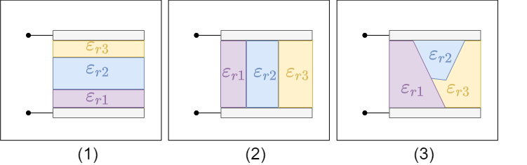
Up to now was assumed only one dielectricum resp. only vacuum within capacitor. Now is looked at more detailed, how multi-layered construction between sheets affects capacity. Thereby several dielectrics build boundary layers between each other. Different variants can be distinguished (figure 37):
- transverse layering: There are different dielectrics perpendicular to the field lines.
Thus, the boundary layers are parallel to the capacitor plates. - Longitudinal layering: There are different dielectrics parallel to the field lines. \ So the boundary layers are perpendicular to the capacitor plates.
- Elongitudinal Stratification: The boundary layers are neither parallel nor perpendicular to the capacitor plates.
Cross-layering
First, the situation is considered that the boundary layers are parallel to the electrode surfaces. A voltage $U$ is applied to the structure from the outside.
The stratification is now parallel to equipotential surfaces. In particular, the boundary layers are then also equipotential surfaces.
The boundary layers can be replaced by an infinitesimally thin conductor layer (metal foil). The voltage $U$ can then be divided into several partial areas:
\begin{align*} U = \int \limits_{total \, inner \\ volume} \! \! \vec{E} \cdot d \vec{s} = E_1 \cdot d_1 + E_2 \cdot d_2 + E_3 \cdot d_3 \tag{5.9.1} \end{align*}
Since there are only polarized charges in the dielectrics and no free charges, the $\vec{D}$ field is constant between the electrodes.
\begin{align*} Q = \iint_{A} \vec{D} \cdot d \vec{A} = const. \end{align*}
Now, in the setup, the area $A$ of the boundary layers is also constant. Thus:
\begin{align*} \vec{D_1} \cdot \vec{A} & = & \vec{D_2} \cdot \vec{A} & = & \vec{D_3} \cdot \vec{A} & \quad \quad \quad & | \vec{D_k} & \parallel \vec{A} \\ D_1 \cdot A & = & D_2 \cdot A & = & D_3 \cdot A & \quad \quad \quad & | \:\: A & = const. \\ D_1 & = & D_2 & = & D_3 & \quad \quad \quad & | D_k & = \varepsilon_{rk} \varepsilon_0 \cdot E_k \\ \varepsilon_{r1} \varepsilon_0 \cdot E_1 &= &\varepsilon_{r2} \varepsilon_0 \cdot E_2 &= &\varepsilon_{r3} \varepsilon_0 \cdot E_3 \\ \end{align*} \begin{align*} \boxed{ \varepsilon_{r1} \cdot E_1 = \varepsilon_{r2} \cdot E_2 = \varepsilon_{r3} \cdot E_3 } \tag{5.9.2} \end{align*}
Using $(5.9.1)$ and $(5.9.2)$ we can also derive the following relationship: \begin{align*} E_2 = & {{\varepsilon_{r1}}\over{\varepsilon_{r2}}}\cdot E_1 , \quad E_3 = {{\varepsilon_{r1}}\over{\varepsilon_{r3}}}\cdot E_1 \\ \end{align*} \begin{align*} U = & E_1 \cdot d_1 + & E_2 & \cdot d_2 + & E_3 & \cdot d_3 \\ U = & E_1 \cdot d_1 + & {{\varepsilon_{r1}}\over{\varepsilon_{r2}}}\cdot E_1 & \cdot d_2 + & {{\varepsilon_{r1}}\over{\varepsilon_{r3}}}\cdot E_1 & \cdot d_3 \\ \end{align*} \begin{align*} U = & E_1 \cdot (d_1 + {{\varepsilon_{r1}}\over{\varepsilon_{r2}}} \cdot d_2 + {{\varepsilon_{r1}}\over{\varepsilon_{r3}}}\cdot d_3 ) \\ E_1 = & {{U}\over{ d_1 + \large{{\varepsilon_{r1}}\over{\varepsilon_{r2}}} \cdot d_2 + \large{{\varepsilon_{r1}}\over{\varepsilon_{r3}}}\cdot d_3 }} \end{align*} \begin{align*} \boxed{ E_1 = {{U}\over{ \sum_{k=1}^n \large{{\varepsilon_{r1}}\over{\varepsilon_{rk}}} \cdot d_k}} } \quad \text{and} \; E_k = {{\varepsilon_{r1}}\over{\varepsilon_{rk}}}\cdot E_1 \end{align*}
The situation can also be transferred to a coaxial structure of a cylindrical capacitor or concentric structure of spherical capacitors.
Merke:
Cross-stratification results in:- A cross-stratification can be considered as a series connection of partial capacitors with respective thicknesses $d_k$ and dielectric constant $\varepsilon_{rk}$.
- The flux density is constant in the capacitor
- Considering the fields along the field line - that is, perpendicular to the interface, or the normal components $E_n$ and $D_n$ of the fields - the following holds:
- The normal component of the electric field strength $E_n$ changes abruptly at the interface.
- The normal component of the flux density $D_n$ is continuous at the interface: $D_{n1} = D_{n2}$
Longitudinal layering
Now the boundary layers should be perpendicular to the electrode surfaces. Again a voltage $U$ is applied to the structure from the outside.
The stratification is now perpendicular to equipotential surfaces. However, the same voltage is applied to each dielectric. Thus it is valid:
\begin{align*} U = \int \limits_{total inner \\ volume} \! \! \vec{E} \cdot d \vec{s} = E_1 \cdot d = E_2 \cdot d = E_3 \cdot d \end{align*}
Since $d$ is the same for all dielectrics, $\large{ E_1 = E_2 = E_3 = {{U}\over{d}} }$
with the displacement flux density $D_k = \varepsilon_{rk} \varepsilon_{0} \cdot E_k$ results:
\begin{align*} { { D_1 } \over { \varepsilon_{r1} } } = { { D_2 } \over { \varepsilon_{r2} } } = { { D_3 } \over { \varepsilon_{r3} } } = { { D_k } \over { \varepsilon_{rk} } } \end{align*}
Since the displacement flux density is just equal to the local surface charge density, the charge will no longer be uniformly distributed over the electrodes.
Where a stronger polarization is possible, the $E$-field is damped in the dielectric. For a constant $E$-field, more charges must accumulate there.
Concretely, more charges accumulate just around the dielectric constant $\varepsilon_{rk}$.
This situation can also be transferred to a coaxial structure of a cylindrical capacitor or concentric structure of spherical capacitors.
Remember:
In the case of longitudinal stratification, the result is:- A longitudinal stratification can be viewed as a parallel connection of partial capacitors with respective areas $A_k$ and dielectric constant $\varepsilon_{rk}$.
- The electric field strength in the capacitor is constant.
- Considering the fields transverse to the field lines - that is, perpendicular to the interface, or the tangential components $E_t$ and $D_t$ of the fields - the following holds:
- The tangential components of the flux density $D_t$ changes abruptly at the interface.
- The tangential components of the electric field strength $E_t$ is continuous at the interface: $E_{t1} = E_{t2}$
any stratification
With arbitrary stratification, simple observation is no longer possible.
However, some hints can be derived from the previous types of stratification:
- Electric field strength $\vec{E}$:
- The normal component $E_{n}$ is discontinuous at the interface: $\varepsilon_{r1} \cdot E_{n1} = \varepsilon_{r2} \cdot E_{n2}$
- The tangential component $E_{t}$ is continuous at the interface: $ E_{t1} = E_{t2}$
- Electric displacement flux density $\vec{D}$:
- The normal component $D_{n}$ is continuous at the interface: $ D_{n1} = D_{n2}$
- The tangent component $D_{t}$ is discontinuous at the interface: $ {{1}\over \Large{\varepsilon_{r1}}\cdot D_{t1} = {{1}\over \Large{\varepsilon_{r2}} \cdot D_{t1} $
Since $\vec{D} = \varepsilon_{0} \varepsilon_{r} \cdot \vec{E}$ the direction of the fields must be the same.
Using the fields, we can now derive the change in the angle:
\begin{align*} \boxed { { { tan \alpha_1 } \over { tan \alpha_2 } } = { { \varepsilon_{r1} } \over { \varepsilon_{r2} } } } \end{align*}
The formula obtained represents the law of refraction of the field line at interfaces. There is also a hint that for electromagnetic waves (like visible light) the refractive index might depend on the dielectric constant. In fact, this is the case. However, in the calculation presented here, electrostatic fields were assumed. In the case of electromagnetic waves, the distribution of energy between the two fields must be taken into account. This is not considered in detail in this course.
Different dielectrics in the capacitor
Tasks
Task 5.9.1 Layered Capacitor Task
Task 5.9.2 Capacitor with glass plate
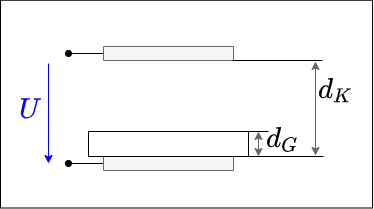
Two parallel capacitor plates face each other with a distance $d_K = 10mm$. A voltage of $U = 3'000V$ is applied to the capacitor. Parallel to the capacitor plates there is a glass plate ($\varepsilon_{r,G}=8$) with a thickness $d_G = 3mm$ in the capacitor.
- Calculate the partial voltages $U_G$ in the glass and $U_L$ in the air gap.
- What is the maximum thickness of the glass pane if the field strength $E_{0,G} =12 kV/cm$ must not exceed.
5.10 Summary
Further links
- Online Bridge Course Physics KIT: This semi-interactive course contains some of the information from my course. Furthermore, videos, exercises and more can be found there
additional Links
Illustrative and interactive examples
A really great introduction in electric and magnetic fields (but a bit too deep for this course) can be found in the physics lectur of Walter Lewin
examples:
8.02x - Lect 1 - Electric Charges and Forces - Coulomb's Law - Polarization
8.02x - Lect 2 - Electric Field Lines, Superposition, Inductive Charging, Induced Dipoles