This is an old revision of the document!
3. The magnetostatic Field
3.1 Magnetic Phenomena
Learning Objectives
By the end of this section, you will be able to:
- Know that forces act between magnetic poles and know the direction of the forces.
- Know that a magnetic field is formed around a current-carrying conductor.
- be able to sketch the field lines of the magnetic field. Know the direction of the field and where the field is densest.
Effects around Permanent Magnets
First permanent magnets made of magnetic magnetite ($Fe_{3} O_{4}$) were found in Greece in the region around Magnesia. Besides the iron materials, other elements also show a similar “strong and permanent magnetic force effect”, which is also called ferromagnetism after iron: Cobalt and nickel, as well as many of their alloys, also exhibit such an effect. Chapter 3.5 Matter in the magnetic field describes the subdivision of magnetic materials in detail.
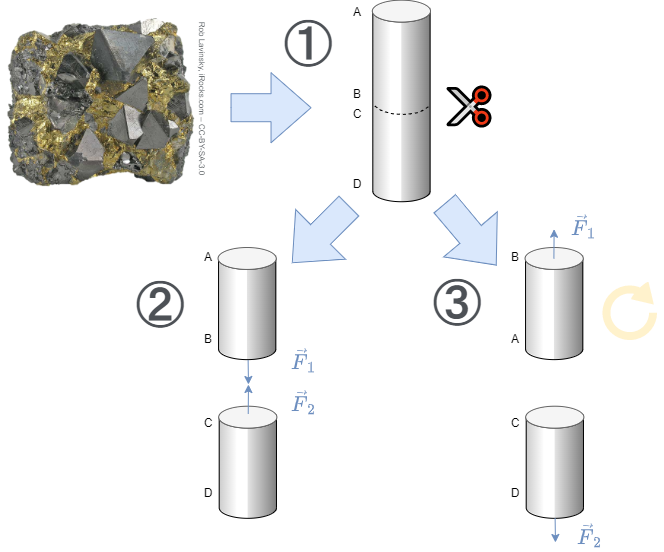
Here now the “magnetic force effect” is to be looked at more near. For this purpose, a few thought experiments are carried out with a magnetic iron stone figure 21 (This video gives a similar introduction).
- From the iron ore should now first be separated a handy elongated part. If one is lucky, the found iron ore is already magnetic by itself. This case will be considered in the following. The elongated piece is now to be cut into two small pieces.
- As soon as the two pieces are removed from each other, one notices that the two pieces attract each other again directly at the cut surface.
- If one of the two parts is turned (the upper part in the picture on the below), a repulsive force acts on the two parts.
So it seems that there is a directed force around each of the two parts. If you dig a little deeper you will find that this force is focused on one part of the outer surface.
Of course you already know magnets and also know that there are poles. The considered thought experiment shall clarify, how one could have proceeded at an unknown appearance. In further thought experiments, such magnet iron stones can also be cut into other directions and the forces analysed.
The result here is:
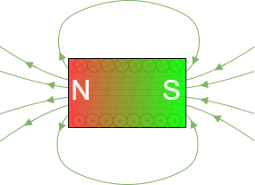
- There are two poles. These are called the north pole and the south pole. The north pole is coloured red, the south pole green.
- Poles with the same name repel each other. Unequal poles attract each other. This is similar to the electric field (opposite charges attract).
- So magnets experience a force in the vicinity of other magnets.
- A compass is a small rotating “sample” magnet and is also called a magnetic needle. This sample magnet can thus represent the effect of a magnet. This is also similar to the sample charge of the electric field.
- The naming of the magnetic poles was done by the part of the compass which points to the geographic north pole. The reason for this is that the magnetic south pole is found at the geographic north pole.
- Magnetic poles are not isolatable. Even the smallest fraction of a magnet shows either no magnetism, or both north and south poles.
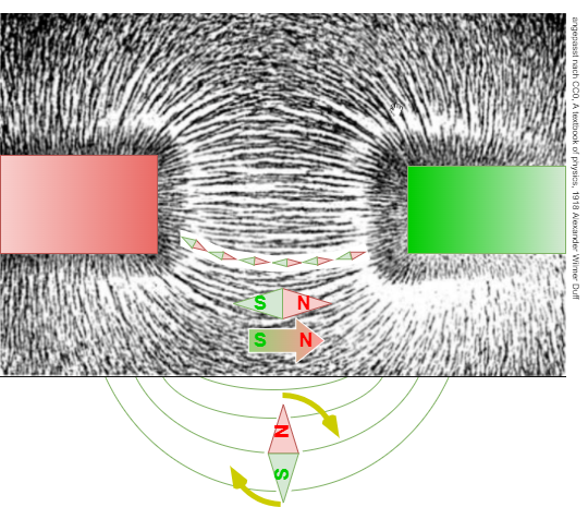
An interesting aspect is that even non-magnetised, ferromagnetic materials experience a force effect in the magnetic field. A non-magnetic nail is attracted by a permanent magnet. This even happens independently of the magnetic pole. This also explains the visualization about iron filings (= small ferromagnetic parts), see figure 2. Also here there is a force effect and a torque, which aligns the iron filings. The visible field seems to form field lines here.
Notice:
- Field line images can be visualized by iron filings. Conceptually, these can be understood as a string of sample magnets.
- The direction of the magnetic field defined via the sample magnet: The north pole of the sample magnet points in the direction of the magnetic field.
- The amount of magnetic field is given by the torque experienced by a sample magnet oriented perpendicular to the field.
- Field lines seem to repel each other (“perpendicular push”). e.g. visible when the field exits the permanent magnet.
- Field lines attempt to travel as short a path as possible (“longitudinal pull”).
Effects around Current-carrying Wires
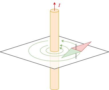
In 1820, Christian Ørsted discovered by chance during a lecture that current-carrying conductors also have an effect on a compass. This experiment is illustrated in figure 3. A long, straight conductor with a circular cross-section has current $I$ flowing through it. Due to symmetry considerations, the field line pattern must be radially symmetric with respect to the conductor axis. By an experiment with a magnetic needle it can be shown that the field lines form concentric circles.
Notice:
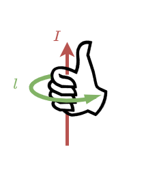
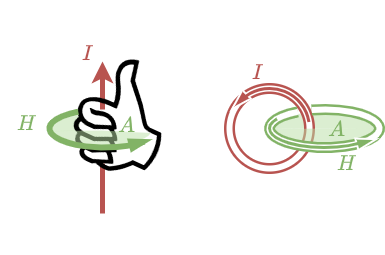
- If the technical direction of current is considered, the magnetic field lines surround the current in the sense of a right hand screw. (“right screw rule”)
- This rule can also be remembered in another way: If the thumb of the right hand points in the (technical) current direction, the fingers of the hand surround the conductor like the magnetic field lines. Likewise, if the thumb of the left hand points in the Electron flow direction, the fingers of the hand surround the conductor like the magnetic field lines.
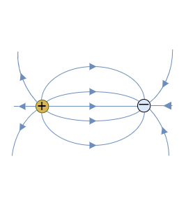
Comparison of Electrostatics and Magnetostatics
3.2 Magnetic Field Strength
Learning Objectives
By the end of this section, you will be able to:
- know the two field-describing quantities of the magnetic field.
- be able to describe and apply the relationship between these two quantities.
Superposition of the magnetostatic Field
Superposition of magnetic fields
Before the magnetic field strength will be considered in more detail, the simulation and superposition of the magnetic field will be discussed in more detail here.
Magnetostatic fields can be superposed, just like electrostatic fields. This allows the fields of several current-carrying lines to be combined into a single one. This trick is used in the following chapter to examine the magnetic field in more detail.
On the right side the magnetic field of a single current-carrying conductor is shown. This was already derived at the previous chapter by symmetry considerations. The representation in the simulation can be simplified a bit here to see the conditions more clearly: Currently, the field lines are displayed in 3D, which is done by selecting “Display: Field Lines” and “No Slicing”. If you change the selection to “Show Z Slice” instead of “No Slicing”, you can switch to a 2D display. In this display, small compass needles can also show the magnetic field. To do this, select “Display: Field Vectors” instead of “Display: Field Lines”. In addition, a “magnetic sample”, i.e. a moving compass, can be found at the mouse pointer in the 2D display.
If there is another current-carrying conductor near the first conductor, the fields overlap. In the simulation on the below, the current of both conductors is directed in the same direction. The field between the conductors overlaps just enough to weaken. This can also be deduced by previous knowledge, if just the middle point between both conductors is considered: There the right hand rule results for the left conductor a vector directed towards the observer. For the right conductor results a vector directed away from the observer. These just cancel each other out. Further outward field lines go around both conductors. North- and south-poles here are not fix localized towards outside.
If, on the other hand, the current in the second conductor is directed in the opposite direction to the current in the first conductor, the picture changes: Here there is a reinforcing superposition between the two conductors. Using the nomenclature from the previous chapter, it is also possible to assign north and south poles locally. Towards the outside, one pole appears to be located in front of the two conductors and another one behind.
in both simulations, the distances between the conductors can also be changed using the “Line Separation” slider. What do you notice in each case when the two lines are brought close together?
Magnetic Field Strength part 1: toroidal Coil
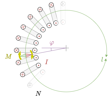
Fig. 6: Magnetic field in a toroidal coil
So far the magnetic field was defined quite pragmatically by the effect on a compass. For a deeper analysis of the magnetic field, the field is now to be considered again - as with the electric field - from two directions. The magnetic field will also be considered as a “causer field” (a field caused by magnets) and an “acting field” (field acting on a magnet). This chapter will first discuss the acting magnetic field. For this, it is convenient to consider the effects inside a toroidal coil (= donut-like setup). This can be seen in figure 6. For reasons of symmetry, it is also clear here that the field lines form concentric circles.
In an experiment, a magnetic needle inside the toroidal coil is now to be aligned at perpendicular to the field lines. Then, the magnetic field will generate a torque $M$ which tries to align the magnetic needle in the field direction.
It now follows:
- $M = const. \neq f(\varphi)$ : For the same distance from the axis of symmetry, the torque $M$ is independent of the angle $\phi$.
- $M \sim I$ : The stronger the current flowing through a winding, the stronger the effect, i.e. the stronger the torque.
- $M \sim N$ : The greater the number $N$ of windings, the stronger the torque $M$.
- $M \sim {1 \over l}$ : The smaller the average coil circumference $l$ the greater the torque. The average coil circumference $l$ is equal to the mean magnetic path length (=average field line length).
To summarize: \begin{align*} M \sim {{I \cdot N}\over{l}} \end{align*}
The magnetic field strength $H$ inside the toroidal coil is given as: \begin{align*} \boxed{H ={{I \cdot N}\over{l}}} \quad \quad | \quad \text{applies to toroidal coil only} \end{align*}
For the unit of the magnetic field strength $H$ we get $[H] = {{[I]}\over{[l]}}= 1{{A}\over{m}}$
Magnetic Field Strength part 2: straight conductor
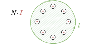
The previous derivation from the toroidal coil is now to be used to derive the field strength around a long, straight conductor. For a single conductor the parte $N \cdot I$ of the formula can be reduced to $ N \cdot I = 1 \cdot I = I$, since there is only one conductor. For the toroidal coil, the magnetic field strength was given by this current(s) divided by the (average) field line length. Because of the (same rotational) symmetry, this is also true for the single conductor. Also here the field line length has to be taken into account.
The length of a field line around the conductor is given by the distance $r$ of the field line from the conductor: $l = l(r) = 2 \cdot \pi \cdot r$.
For the magnetic field strength of the single conductor we then get:
\begin{align*}
\boxed{H ={I\over{l}} = {{I}\over{2 \cdot \pi \cdot r}}} \quad \quad | \quad \text{applies only to the long, straight conductor}
\end{align*}
In the electric field, the field line density was a measure of the strength of the field. This is also used for the magnetic field. Looking at the simulations in Falstad (e.g. figure 8) with this understanding, one notices an inconsistency: contrary to the relationship just given, the field line density in the Falstad simulation not indicates the strength of the field. A realistic simulation is shown in figure 9 for comparison, which makes the difference clear: the field is stronger near the conductor. Thus the field line density must also be stronger there.
Attention:
- The density of the field lines is a measure of the field strength.
- The simulation in Falstad cannot represent this in this way. Here the field strength is coded by the color intensity (dark green = low field strength, light green to white = high field strength).
Magnetic Voltage
The cause of the magnetic field is the current. As seen for the coil, sometimes the current have to be counted up ($N \cdot I$), e.g. by the number of windings of the coil. If this current $I$ and/or the number $N$ of windings is increased, the effect is amplified. To make this easier to handle, we introduce the Magnetic Voltage. The magnetic voltage $\theta$ is defined as
\begin{align*} \boxed{\theta = \sum I = N \cdot I} \end{align*} The unit of $\theta$ is: $[\theta]= 1A$ (obsoletely called ampere-turn). For the magnetic voltage the currents which flow through the surface enclosed by the closed path have to be considered. A detailed definition will be given below after more analysis.
Thus, the magnetic field strength $H$ of the toroidal coil is then given by: $H= {{\theta}\over{l}}$
Notice:
- For the sign of the magnetic voltage, one has to consider the orientation of the current and way on the enclosing path. The figure 10 shows the positive orientation: The positive orientation is given, when the currents show out of the drawing plane and the path shows a counter clockwise orientation.
- This is again given as the right hand rule (see figure 11): For the positive orientation the current shows along the thumb of the right hand, while the path is counted along the direction of the fingers of the right hand.
In the English literature often the name Magnetomotive Force $\mathcal{F}$ is used instead of magnetic voltage $\theta$. The naming refers to the Electromotive Force, which depicts the ability of a voltage source to be able to drive a current in order to build a a defined voltage. Both “forces” shall not be confused with the mechanical force $\vec{F}= m \cdot \vec{a}$. They only describe the driving cause behind the electric or magnetic fields. The German courses in higher semesters use the term “Magnetische Spannung” - therefore, the English equivalent is introduced here.
Magnetic Field Strength part 3: Generalization
So far, only rotationally symmetric problems could be solved. Now this shall be generalized. For this purpose we will have a look back to the electric field. For the electric field strength $E$ of a capacitor with two plates at a distance of $s$ and the potential difference $U$ holds:
\begin{align*} U = E \cdot s \quad \quad | \quad \text{applies to capacitor only} \end{align*}
In words: The potential difference ifs given by adding up the field strength along the path of a probe from one plate to the other. This was extended to $U = \int_s E ds$. If we pompare this idea to the magnetic field strength $H$ of a toroidal coil with the mean magnetic path length $l$, we had
\begin{align*} \theta = H \cdot l \quad \quad | \quad \text{applies to toroidal coil only} \end{align*}
Can you see the similarities? Again, the magnitude of the field strength is summed up along a path to arrive at another field-describing quantity (here, the magnetic voltage $\theta$). Because of the similarity - which continues below - the so-called magnetic potential difference $V_m$ is introduced:
\begin{align*} V_m = H \cdot s \quad \quad | \quad \text{applies to toroidal coil only} \end{align*}
Now what is the difference between the magnetic potential difference $V_m$ and the magnetic voltage $\theta$?
- The first equation of the toroidal coil ($\theta = H \cdot l$) is valid for exactly one turn along a field line with the length $l$. In addition, the magnetic voltage was equal to the current times the number of windings: $\theta = N \cdot I$.
- The second equation ($V_m = H \cdot s$) is independent of the length of the field line $l$. Only if $s = l$ is chosen, the magnetic voltage equals the magnetic potential difference. The path length $s$ can be a fraction or multiple of a single revolution $l$ for the magnetic potential difference.
Thus, for each infinitesimally small path $ds$ along a field line, the resulting infinitesimally small magnetic potential difference $dV_m = H \cdot ds$ can be determined. If now along the field line the magnetic field strength $H = H(\vec{s})$ changes, then the magnetic potential difference from point $\vec{s_1}$ to point $\vec{s_2}$ results to:
\begin{align*} V_{m12} = V_m(\vec{s_1}, \vec{s_2}) = \int_\vec{s_1}^\vec{s_2} H(\vec{s}) ds \end{align*}
Up to now only the situation was considered that one always walks along one single field line. $\vec{s}$ therefore always arrived at the same spot of the field line. If one wants to extend this to arbitrary directions (also perpendicular to field lines), then only that part of the magnetic field strength $\vec{H}$ may be used in the formula, which is parallel to the path $d \vec{s}$. This is made possible by scalar multiplication. Thus, it is generally valid:
\begin{align*} \boxed{V_{m12} = \int_\vec{s_1}^\vec{s_2} \vec{H} \cdot d \vec{s}} \end{align*}
The magnetic voltage $\theta$ (and therefore the current) is the cause of the magnetic field strength. From the chapter The stationary Electric Flow the general representation of the current through a surface is known. This leads to the Ampere's Circuital Law
\begin{align*} \boxed{\int_{closed \\ path} \vec{H} \cdot d \vec{s} = \iint_{enclosed \\ surface \; A} \vec{S} d\vec{A} = \theta} \end{align*}
- The path integral of the magnetic field strength along an arbitrary closed path is equal to the free currents (= current density) through the surface enclosed by the path.
- The magnetic voltage $\theta$ can be gib
- for a single conductor: $\theta = I$
- for a coil: $\theta = N \cdot I$
- for multiple conductors: $\theta = \sum_n \cdot I_n$
- for spatial distribution: $\theta = \iint_{enclosed \\ surface \; A} \vec{S} d\vec{A}$
- $d\vec{s}$ and $d\vec{A}$ build a right hand system: once the thumb of the right hand is pointing along $d\vec{A}$, the fingers of the right hand show the correct direction for $d\vec{s}$ for positive $\vec{H}$ and $\vec{S}$
Recap: Application of magn. Field Strength
The Ampere's Circuital Law shall be applied in order to find the magnetic field strength $H$ inside the toroidal coil (figure 13).
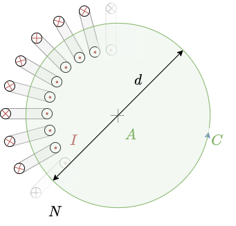
- The closed path $C$ is on revolution of a field line in the center of the coil
- the surface $A$ is the enclosed surface
This leads to:
\begin{align*} \int_C \vec{H} \cdot d \vec{s} &= \iint_{A} \vec{S} d\vec{A} = \theta \end{align*}
Since $\vec{H} \uparrow \uparrow d \vec{s}$ the term $\vec{H} \cdot d \vec{s}$ can be substituted by $H ds$:
\begin{align*} \int_C H \cdot ds &= \iint_{A} \vec{S} d\vec{A} \end{align*}
The magnetic voltage is the current through the surface and given as $N\cdot I$:
\begin{align*} \int_C H \cdot ds &= N\cdot I \end{align*}
The magnetic field strength $H$ can be considered constant:
\begin{align*} H \cdot \int_C ds &= N\cdot I \end{align*}
The average coil circumference is $2\pi \cdot {{d}\over{2}}$:
\begin{align*} H \cdot 2\pi \cdot {{d}\over{2}} &= N\cdot I \end{align*}
Therefore, the magnetic field strength in the toroidel coil is \begin{align*} H &= {{N\cdot I}\over{ \pi \cdot d }} \end{align*}
Similarly, the magnetic field strength $H$ in the distance $r$ to a single conductor with the current $I$ can be derived. In this situation the result is:
\begin{align*} H &= {{I}\over{ 2\pi \cdot r }} \end{align*}
3.3 Magnetic Flux Density and Lorentz Law
Learning Objectives
By the end of this section, you will be able to:
- know the force law for current-carrying conductors.
- Be able to determine the direction of the forces using given current directions and, if applicable, flux density.
- be able to represent the vectors of the magnetic flux density in a sketch when several current-carrying conductors are specified.
- be able to determine a force vector by superimposing several force vectors using vector calculus.
- be able to state the following quantities for a force vector on a current-carrying conductor in a magnetostatic field:
- Force vector in coordinate representation
- magnitude of the force vector
- Angle of the force vector
Definition of the Magnetic Flux Density
In the last subchapter the field effect on a magnet caused by currents was analyzed. Now, the field acting onto currents will get deeper investigation. In order to do so, the effect between two parallel conductors has to be examined closer. The experiment consists of a part $l$ of two very long1) conductors with the differenct currents $I_1, I_2$ in the distance $r$ (see figure 14).
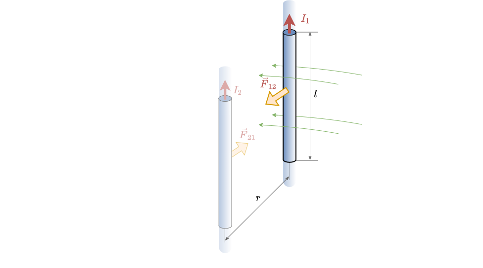
When no current is flowing through the conductors the forces er equal to zero. Once the currents flow in the same direction (e.g. $I_1>0, I_2>0$) attracting forces $\vec{F}_{12} = - \vec{F}_{21}$ appear. The force $\vec{F}_{xy}$ shall be the force on the conductor $x$ caused by conductor $y$. In the following the force $\vec{F}_{12}$ on the conductor $1$ will be examined.
The following is detectable:
- $|\vec{F}_{12}| \sim I_1$, $|\vec{F}_{12}| \sim I_2$ : The stronger each current, the stronger the force $F_{12}$.
- $|\vec{F}_{12}| \sim l$ : As longer the conductor length $l$, as stronger the force $F_{12}$ gets.
- $|\vec{F}_{12}| \sim {{1}\over{r}}$ : A smaller distance $r$ leads to stronger force $F_{12}$.
To summarize: \begin{align*} {F}_{12} \sim {I_1 \cdot I_2 \cdot {{l}\over{r}}} \end{align*}
The proportionality factor is arbitrarily chosen as: \begin{align*} {{{F}_{12} \cdot r} \over {I_1 \cdot I_2 \cdot {l}}} = {{\mu}\over{2\pi}} \end{align*}
Here $\mu$ is the magnetic permeability and for vacuum (vacuum permeability): \begin{align*} \mu = \mu_0 = 4\pi \cdot 10^{-7} {{Vs}\over{Am}} = 1.257 \cdot 10^{-7} {{Vs}\over{Am}} \end{align*}
This leads to the Ampere's Force Law: \begin{align*} |\vec{F}_{12}| = {{\mu}\over{2 \pi}} \cdot {{I_1 \cdot I_2 }\over{r}} \cdot l \end{align*}
Since we want to investigate the effect onto the current $I_1$, the following rearrangement can be done: \begin{align*} |\vec{F}_{12}| &= {{\mu}\over{2 \pi}} \cdot {{I_2 }\over{r}} &\cdot I_1 \cdot l \\ &= B &\cdot I_1 \cdot l \\ \end{align*}
The properties of the field from $I_2$ acting on $I_1$ is summarized to $B$ - the magnetic flux density. $B$ has the unit: \begin{align*} [B] &= {{[F]}\over{[I]\cdot[l]}} = 1 {{N}\over{Am}} = 1 {{{VAs}\over{m}}\over{Am}} = 1 {{Vs}\over{m^2}} \\ &= 1 T \quad\quad(Tesla) \end{align*}
This formula can be generalized with the knowledge of the directions of the conducting wire $\vec{l}$, the magnetic field strength $\vec{B}$ and the force $\vec{F}$ by means of vector mutiplication to:
\begin{align*} \boxed{\vec{F_L} = I \cdot \vec{l} \times \vec{B}} \end{align*}
The absolute value can be calculated by
\begin{align*} \boxed{|\vec{F_L}| = I \cdot |l| \cdot |B| \cdot sin(\angle \vec{l},\vec{B} )} \end{align*}
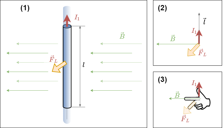
The force is often called Lorentz Force $F_L$. For the orientation another right hand rule can be applied.
Notice:
Right hand rule for the Lorentz Force:- The causing current $I$ is on the thumb. Since the current is not a vector, the direction is given by the direction of the conductor $\vec{l}$
- The mediating external magnetic field $\vec{B}$ is on the index finger
- The resulting force $\vec{F}$ on the conductor is on the middle finger
This is shown in figure 14.
A way to remember the orientation is the mnemonic FBI (from middle finger to thumb):
- $\vec{F}$orce on middle finger
- $\vec{B}$-Field on index finger
- Current $I$ on thumb (direction with length $\vec{l}$)
Lorentz Law and Lorentz Force
The true Lorentz force is not the force on the whole conductor but the single force onto a (elementary) charge.
In order to find this force the previous force onto a conductor can be used as a start. However, the formula will be investigated infinidesimally for small parts $d \vec{l}$ of the conductor:
\begin{align*} \vec{dF}_L = I \cdot d\vec{l} \times \vec{B} \end{align*}
The current is now substituted by $I = dQ/dt$, where $dQ$ is the small charge packet in the length $\vec{dl}$ of the conductor.
\begin{align*} \vec{dF}_L = {{dQ}\over{dt}} \cdot d\vec{l} \times \vec{B} \end{align*}
Mathematically not quite correct, but in a physical way true the following rearrangement can be done:
\begin{align*} \vec{dF}_L &= {{dQ \cdot d\vec{l}}\over{dt}} \times \vec{B} \\ &= dQ \cdot {{d\vec{l}}\over{dt}} \times \vec{B} \\ &= dQ \cdot {{d\vec{l}}\over{dt}} \times \vec{B} \\ \end{align*}
Here, the part ${{d\vec{l}}\over{dt}}$ represents the speed $\vec{v}$ of the small charge packet $dQ$.
\begin{align*} \vec{dF}_L &= dQ \cdot \vec{v} \times \vec{B} \end{align*}
The Lorenz Force on a finite charge packet is the integration:
\begin{align*} \boxed{\vec{F}_L = Q \cdot \vec{v} \times \vec{B}} \end{align*}
Notice:
- A charge $Q$ moving with a velocity $\vec{v}$ in a magnetic field $\vec{B}$ experiences a force of $\vec{F_L}$.
- The direction of the force is given by the right hand rule.
Please have a look at the contents (text, videos, exercises) on the page of the KIT-Brückenkurs >> 5.2.3 Lorentz-Kraft. Make sure that “Gesamt” is selected in the selection bar at the top. The last part on “Magnetic field with matter” can be skipped.
3.4 Matter in the Magnetic Field
Learning Objectives
By the end of this section, you will be able to:
- know the two field-describing quantities of the magnetostatic field.
- be able to describe and apply the relationship between these two quantities via the material law.
- know the classification of magnetic materials.
- be able to read the relevant data from a magnetisation characteristic curve.
The magnetic interaction are also represented via two fields in the previous subchapters similar to the electric field.
Since the magnetic field strength $\vec{H}$ is only depending on the field causing current $I$, this field is independent from surrounding matter.
The magnetic flux density $\vec{B}$ on the other hand, showed with the magnetic permeability a factor which can contain the material effects.
Both fields are connected. The Ampere's Force Law gave the formula
\begin{align*} |\vec{F}_{12}| &= {{\mu}\over{2 \pi}} \cdot {{I_2 }\over{r}} &\cdot I_1 \cdot l \\ &= B &\cdot I_1 \cdot l \\ \end{align*}
Therefore, the magnetic flux density $\vec{B}$ is equal to:
\begin{align*} B &= {{\mu}\over{2 \pi}} \cdot {{I_2 }\over{r}} \end{align*}
$I_2$ was here the field-causing current.
For the field strength of the straight conductor we had:
\begin{align*} H &= {{I}\over{2 \pi \cdot r }} \end{align*}
The connection between the two field is also $B = \mu \cdot H$ . Since the field lines of borth fields are always parallel to each other it results to
\begin{align*} \boxed{ \vec{B} = \mu \cdot \vec{H} } \end{align*}
This is similar to the $\vec{D} = \varepsilon \cdot \vec{E}$. Similarly, the permeability is separated into two parts:
\begin{align*} \mu &= \mu_0 \cdot \mu_r \end{align*}
where
- $\mu_0$ is the permeability of the vacuum
- $\mu_r$ is the relative permeability, for the case that there is material in the magnetic field
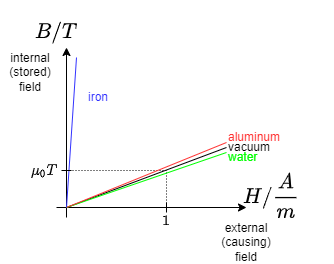
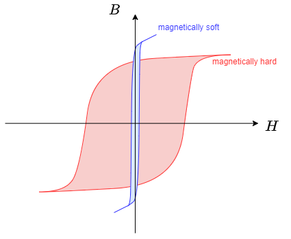
The material can be divided into different types by looking onto their relative permeability. figure 16 shows the relative permeability in the magnetization curve (also called $B$-$H$-curve). In this diagram the different effect ($B$-field on $y$-axis) based on the causing external $H$-field (on $x$-axis) for different materials is shown. The three most important material types shall be discussed shortly.
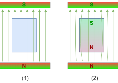
Diamagnetic Materials
- Diamagentic materials weaken the magnetic field, compared to the vacuum.
- The weakening is very low (see table 1).
- For diamagnetic materials applies $0<\mu_r<1$
- The principle behind the effect is based on quantum mechanics (see figure 17):
- Without the external field no counteracting field is generated by the matter.
- With an external magnetic field an antiparallel orientated magnet is induced.
- The reaction weakens the external field. This is similar to weakening of the elektric field by the dipoles of materials.
- Due to the repulsion of the outer magnetic field the material tend to move out of a magnetic field.
For very stron magnetic fields small objects can be levitated (see clip).
A living insect (“diamagnet”) floats in a very strong magnetic field
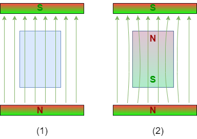
Paramagnetic Materials
- Paramagentic materials strengthen the magnetic field, compared to the vacuum.
- The strengthening is very low (see table 2).
- For paramagnetic materials applies $\mu_r>1$
- The principle behind the effect is again based on quantum mechanics (see figure 18):
- Without the external field no counteracting field is generated by the matter.
- With an external magnetic field internal “tiny magnets” based on the electrons in their orbitals are orientated similarly.
- This reaction strengthen the external field.
Explanation of diamagnetism and paramagnetism
Ferromagnetic Materials
- Ferromagentic materials strengthen the magnetic field strongly, compared to the vacuum.
- The strengthening can create a field multiple times stronger than in vacuum.
- For ferromagnetic materials applies $\mu_r \gg 1$
- The principle behind the effect is based on quantummechanics:
- Also here internal “tiny magnets” based on the electrons in their orbitals are oriented based on the external field.
- However, these “tiny magnets” ineract with each other in such a way that the field becomes stable even without the external field.
- Ferromagnetic materials can be permanently magnetized. They build up permanent magnets.
- The magnetic flux density of the ferromagnetic matter is depending on the external field strength and the history of the material.
- The dependency between $\mu_r$ and the external field strength $H$ is nonlinear.
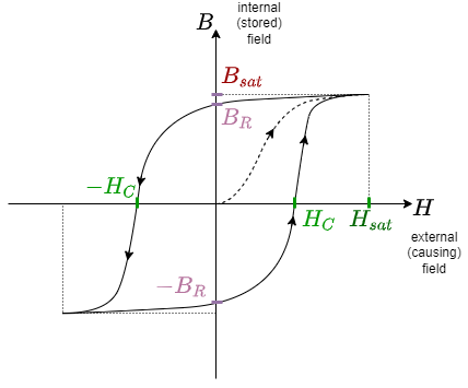
- Ferromagnetic materials are characterized by the magnetization curve (see figure 19)
- Non-magnetized ferromagnets are located in the origin.
- With an external field $H$ the initial magnetization curve (in German: Neukurve, dashed in figure 19) is passed.
- Even without an external field ($H=0$) and the internal field is stable.
The stored field without external field is called remanence $B(H=0) = B_R$ (or remanent magnetization). - In order to eliminate the stored field the counteracting coercive field strength $H_C$ (also called coercivity) has to be applied.
- The saturation flux density $B_{sat}$ is the maximum possible magnetic flux density (at the maximum possible field strength $H_{sat}$)
Explanation of the hysteresis curve
The ferromagnetic materials can again be subdividided into two groups: magnetically soft and magnetically hard materials.
magnetically soft ferromagnetic Materials
- high permeability
- high saturation flux density $B_{sat}$ (= good magnetic conductor)
- small coercive field strength $H_C < 1 kA/m$ (= easy to reverse the magnetization)
- low magnetic losses for reversing the magnetization
- Important materials: ferrites
Applications:
- mainly for coil core material
- rotor and stator material for electric motors
magnetically hard ferromagnetic Materials
- low permeability
- low saturation flux density $B_{sat}$ (= good magnetic conductor)
- high coercive field strength $H_C$ up to $2700 kA/m$ (= easy to reverse the magnetization)
- high magnetic losses for reversing the magnetization
Applications:
- mainly for permanent magnets
- permanent electric motors
- loudspeakers and microphones
- mechanical actuators
Wandering magnetic domains in a ferromagnetic material when the external field is reversed (from [email protected]).
3.5 Poynting Vector (not part of the curriculum)
- Clear picture of the Poynting vector along an electric circuit: https://de.cleanpng.com/png-jyy1vj/
- Good explanation of the Energy flow via a current model: http://amasci.com/elect/poynt/poynt.html
- Very detailed view of the energy flow in an electric circuit: http://sharif.edu/~aborji/25733/files/Energy%20transfer%20in%20electrical%20circuits.pdf
Tasks
Task 3.2.1 Magnetic Field Strength around a horizontal straight Conductor
The current $I = 100A$ flows in a long straight conductor with a round cross-section. The radius of the conductor is $r_{L}= 4mm$.
- What is the magnetic field strength $H_1$ at a point $P_1$, which is outside the conductor at a distance of $r_1 = 10cm$ from the conductor axis?
- What is the magnetic field strength $H_2$ at a point $P_2$, which is inside the conductor at a distance of $r_2 = 3mm$ from the conductor axis?
Task 3.2.2 Superposition
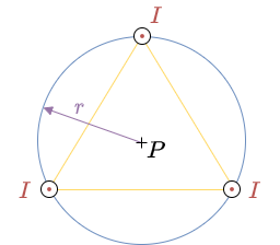
Three long straight conductors are arranged in a vacuum so that they lie at the vertices of an equilateral triangle (see figure 21). The radius of the circumcircle is $r = 2 cm$; the current is given by $I = 2A$.
- What is the magnetic field strength $H(P)$ at the center of the equilateral triangle?
- Now, the current in one of the conductors is reversed. To which value the magnetic field strength $H(P)$ changes?
Task 3.2.3 Magnetic Voltage
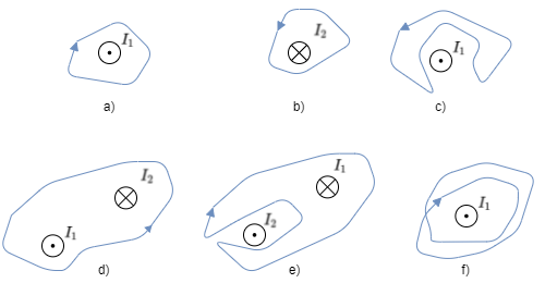
Given are the adjacent closed trajectories in the magnetic field of current-carrying conductors (see figure 10). Let $I_1 = 2A$ and $I_2 = 4.5A$ be valid.
In each case, the magnetic voltage $V_m$ along the drawn path is sought.
Task 3.3.1 magnetic Flux Density
A NdFeB-magnet can show a magnetic flux density up to $1.2 T$ near to the surface.
- For comparison the same flux density shall be created in the inside of a toroidal coil with $10'000$ windings and a toroid diameter for the average field line of $d = 1m$.
How much current $I$ is necessary in one of the windings of the toroidal coil? - What would be the current $I_{Fe}$m when a iron core with $\varepsilon_{Fe,r} = 10'000$?
Task 3.3.2 Electron in Plate Capacitor with magnetic Field
An electron shall move with the velocity $\vec{v}$ in a plate capacitor parallel to the plates, which have a potential difference $U$ and a distance $d$. In the vacuum in between the plates acts additionally a magnetic field $\vec{B}$.
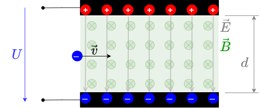
![[email protected]](https://en.wikipedia.org/wiki/Ferromagnetism#/media/File:Moving_magnetic_domains_by_Zureks.gif)
Calculate the velocity depending on the other parameters $\vec{v} = f(U, |\vec{B}|, d) $!
\begin{align*} \vec{F}_C = q_e \cdot \vec{E} \end{align*}
Within the magnetic field the Lorentz force acts on the electron:
\begin{align*} \vec{F}_L = q_e \cdot \vec{v} \times \vec{B} \end{align*}
The absolute value of both forces must be equal in order to compensate each other out:
\begin{align*} |\vec{F}_C| &= |\vec{F}_L|\\ |q_e \cdot \vec{E}| &= |q_e \cdot \vec{v} \times \vec{B}| \\ q_e \cdot |\vec{E}| &= q_e \cdot |\vec{v} \times \vec{B}| \\ |\vec{E}| &= |\vec{v} \times \vec{B}| \\ \end{align*}
Since $\vec{v}$ is perpendicular to $\vec{B}$ the right side is equal to $|\vec{v}| \cdot |\vec{B}| = v \cdot B$.
Additionally, for the plate capacitor $|\vec{E}|= U/d$.
Therefore, it leads to:
\begin{align*} {{U}\over{d}} &= v \cdot B \\ v &= {{U}\over{B \cdot d}} \end{align*}
Task 1
- References to the media used