This is an old revision of the document!
2. The stationary Current Density and Flux
At the dissusion of the electrostatic field in principle no charges in motion were considered. Now the motion of charges shall be considered explicitly.
The current density here describes how charge carriers move together (collectively). The stationary current density describes the charge carrier movement, if a direct voltage is the cause of the movement. A constant direct current then flows in the stationary electric flow field. Thus there is no time dependence of the current:
$\large{{dI}\over{dt}}=0$
Also important is: Up to now was considered, charges did move through a field or could be moved in future. Now just the moment of the movement is considered.
2.1 Current Strength and Flux Field
Goals
After this lesson, you should:
- be able to sketch the flux field in a constricted and rectilinear conductor.
- Be able to determine the flow velocity of electrons.
- know the integral notation of the electric current.
Current and current density in a Simple Case
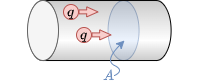
The current strength was previously understood as “charge per time” ($I={{dQ}\over{dt}}$). Microscopically, electric current is the directed motion of electric charge carriers. In the chapter Basic concepts we have already discussed the picture of the charge carrier current penetrating through a cross-sectional area $A$ (see figure 1). Furthermore, we had quite practically applied Ohm's law with $R = {{U}\over{I}}$ in DC. Now we know that the voltage in a electrostatic field can be derived from the electric field strength. But what about the current?
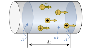
For this purpose, a packet of charges $dQ$ is considered, which will pass the area $A$ during the period $dt$ (see figure ##). These charges are located in a partial volume element $dV$, which is given by the area $A$ to be traversed and a partial section $dx$: $dV = A \cdot dx$. The amount of charges per volume is given by the charge carrier density, specifically for metals by the electron density $n_e$. The electron density $n_e$ gives the number of free electrons per unit volume a. For copper, for example, this is approximately $n_e(Cu)=8.47 \cdot 10^{19} {{1}\over{mm^3}}$.
Fig. 2: Charges in a partial volume in the conductor
. 
The flowing charges contained in the partial volume element $dV$ are then (with elementary charge $e_0$):
\begin{align*} dQ = n_e \cdot e_0 \cdot A \cdot dx \end{align*}
The current is then given by $I={{dQ}\over{dt}}$:
\begin{align*} dQ = n_e \cdot e_0 \cdot A \cdot {{dx}\cdot{dt}} = n_e \cdot e_0 \cdot A \cdot v_e \end{align*}
This leads to an electron velocity $v_e$ of:
\begin{align*} v_e = {{dx}\cdot{dt}} = {{I}\over{n_e \cdot e_0 \cdot A }} \end{align*}
In contrast to the considerations in electrostatics, the charges now travels with finite velocities. With regard to the electron velocity $v_e \sim {{I}\over{A}}$ it is obvious to determine a current density $S$ (related to the area):
\begin{align*} \boxed{S = {{I}\over{A}}} \end{align*}
In some books, the letter $J$ is alternatively used for current density.
Field lines and Equipotential Surfaces of the Current Density
The values of the current density can be given for any point in space. Therefore, the current density can also be considered as a field. As with the electrostatic field, a homogeneous field form and the inhomogeneous field form are to be contrasted:
- In a homogeneous current field (e.g. conductor with constant cross-section) the field lines of the current run parallel. The equipotential surfaces are always perpendicular to each other, because the potential energy of a charge depends only on its position along the path.
Additionally, the equipotential surfaces are equidistant due to the homogeneous geometry and the constant electric field , which causes the current.
Therefore the current $I = S \cdot A$ is constant
$\rightarrow$ the charge carriers have the same velocity $v$
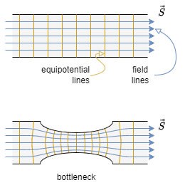
- In an inhomogeneous current field (e.g. a fuse or bottleneck in a wire) the field lines of the current are not parallel. the current $I = S \cdot A$ along the wire must also be constant, because the charge does not disappear or appear from nothing, but the area $A$ becomes smaller.
$\rightarrow$ thus the current density $S$ and the velocity $v$ at the bottleneck must become larger.
The equipotential surfaces are again perpendicular to the current density. The current does now show a compression at the bottleneck.
But why is there a compression of the equipotential surfaces at a bottleneck (see figure 3)?
This means that there is a large potential difference, i.e. a large voltage. So, this already sounds a little bit plausible. This will be looked at in more detail in a moment.
Fig. 3: Field Lines and equipotential Surfaces of the electric Current Field
The current density was determined only for a constant cross-sectional area $A$, through which a homogeneous current - thus also a homogeneous current field - passes at perpendicularly. Now however, a general approach for the electric current strength has to be found.
For this purpose, instead of a constant current density $S$ over a vertical, straight cross-sectional area $A$, a varying current density $S(A)$ over many small partial areas $dA$ is considered. Thus, if the subareas are sufficiently small, a constant current density over the subarea can again be obtained. It then becomes
\begin{align*} I = S \cdot A \rightarrow dI = S \cdot dA \end{align*}
The total current over a larger area $A$ is thus given as:
\begin{align*} I = \int dI = \iint_A S \cdot dA \end{align*}
But what was not considered here: The chosen area $A$ does not necessarily have to be perpendicular to the current density $S$. To take this into account, the (partial) surface normal vector $d\vec{A}$ can be used. If only the part of the current density $\vec{S}$ is to be considered which acts in the direction of $d\vec{A}$, this can be determined via the scalar product:
\begin{align} I = \int dI = \iint_A \vec{S} \cdot d\vec{A} \end{align}
This represents the integral notation of the electric current strength. This can be used to determine the current strength in any field. The current $I$ is the flux of the current density vector $\vec{S}$.
General Material Law
For a “pragmatic” derivation of the general material law for the current density, the compression of the equipotential surfaces at the constriction shall be discussed again. Between two equipotential surfaces there is a voltage difference $\Delta U$. If one chooses this sufficiently small, the transition of $\Delta U \rightarrow dU$ results again. However, the same current $I$ must always flow through the potential surfaces in the conductor. Ohm's law then gives the partial resistance $dR$ between the two equipotential surfaces:
\begin{align*} dU = I \cdot dR \tag{2.1.1} \end{align*}
The individual quantities are now to be considered for infinitesimally small parts. For $I$ an equation about a density - the current density - was already found:
\begin{align*} I = S \cdot A \tag{2.1.2} \end{align*}
But also $R$ has already been expressed by a “density” - the resistivity $\varrho$: $ R = \varrho \cdot {{l}\over{A}}$
If a conductor made of the same material is considered, the resistivity $\varrho$ is the same everywhere. But if there is now a partial element $ds$ along the conductor, where the cross-section $A$ is smaller, the resistance $dR$ of this partial element also changes. The partial resistance is then:
\begin{align*} dR = \varrho \cdot {{ds}\over{A}} \tag{2.1.3} \end{align*}
In concrete terms, this means for the bottleneck: The resistance increases at the bottleneck. Thus the voltage drop also increases there. Thus there are also more equipotential surfaces there.
This solves the question, why there is a compression of the equipotential surfaces at the bottleneck (cmp. figure ##). Interestingly, the thought model can now also for a homogeneous body explain the general material law. To do this, one inserts equation $(2.1.2)$ and $(2.1.3)$ into $(2.1.1)$. Then it follows:
\begin{align*} dU = I \cdot dR = S \cdot A \cdot \varrho \cdot {{ds}\over{{A}}} = \varrho \cdot S \cdot ds \\ \end{align*}
If now the electric field strength is inserted as $E={{dU}\over{ds}}$, one obtains:
\begin{align*} E = {{dU}\over{ds}} = \varrho \cdot S \end{align*}
With a more detailed (and mathematically correct) derivation you get:
\begin{align*} \boxed{\vec{E} = \varrho \cdot \vec{S} } \end{align*}
This equation expresses how the electric field $\vec{E}$ and the (stationary) current density $\vec{S}$ are related: both point in the same direction. For a given electric field $\vec{E}$ in a homogeneous conductor, the smaller the resistivity $\varrho$, the larger the current density $\vec{S}$.
Tasks
Task 2.1.1 calculated exercises in video
Examples of electrical current density
Task 2.1.2 Electron velocity in copper
In a conductor made of copper with cross-sectional area $A$, the current $I = 20A$ flows.
Let further be given the electron density $n_e(Cu)=8.47 \cdot 10^{19} {{1}\over{mm^3}}$ and the magnitude of the elementary charge $e_0 = 1.602 \cdot 10^{-19} As$
- What is the average flow velocity $v_{e,1}$ of electrons when the cross-sectional area of the conductor is $A = 1.5mm^2$?
- What is the average flow velocity $v_{e,1}$ of the electrons when the cross-sectional area of the conductor is $A = 1.0mm^2$?
2.2 Gauss's Law for Current Density
Targets
After this lesson, you should:
- know which quantities are comparable for the electrostatic field and the flow field.
- be able to explain the displacement current on the basis of enveloping surfaces.
- understand how current can flow “through” a capacitor.
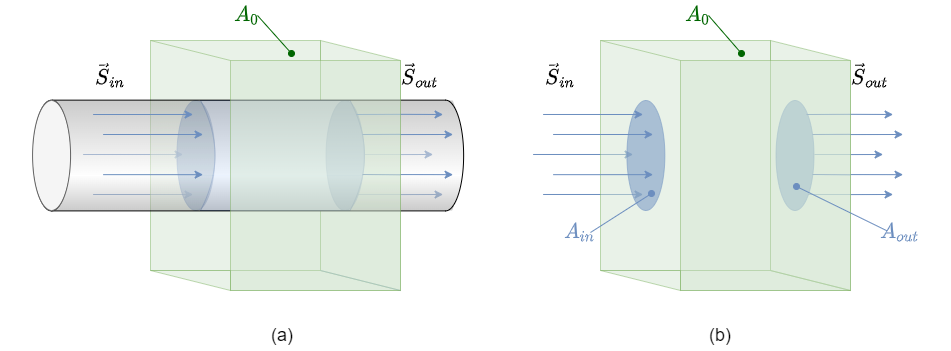
On can now compare the formulas of the current density with the formulas of the displacement flux density. Interestingly, these have a similar structure (see figure ##). However, the Gauss's law for the current density was not considered up to now.
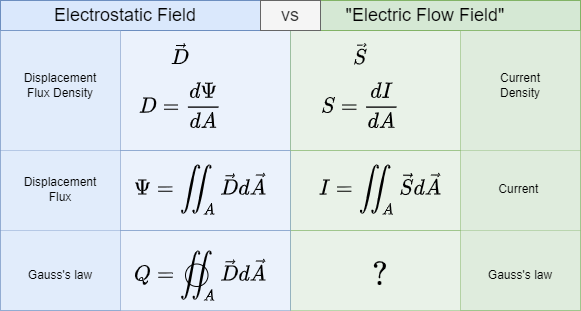
The Gauss's law of the current density shall be analyzed now. figure 5 shows a closed surface around a part of the wire. Since the charge has to be conserved, the incoming current $I_{in}= S_{in}\cdot A_{in}= {{dQ_{in}}\over{dt}}$ must be equal to the outgoing current $I_{out}= S_{out}\cdot A_{out}= {{dQ_{out}}\over{dt}}$
Why does an electron “flow” through a capacitor?
Tasks
Task 2.2.1 Simulation
In the simulation program of Falstad can be represented by equipotential surfaces, electric field strength and current density in different objects.
- Open the simulation program via the link
- Select: “Setup: Wire w/ Current” and “Show Current (j)”.
- You will now see a finite conductor with charge carriers starting at the top end and arriving at the bottom end.
- We now want to observe what happens when the conductor is tapered.
- To do this, select “Mouse = Clear Square”. You can now use the left mouse button to remove parts from the conducting material. The aim should be, that in the middle of the Conductor there is only a one box wide line, on a length of at least 10 boxes. If you want to add conductive material again, this is possible with “Mouse = Add - Conductor”.
- Consider why more equipotential lines are now accumulating as the conductor is tapered.
- If you additionally draw in the E-field with “Show E/j”, you will see that it is stronger along the taper. This can be checked with the slider “Brightness”. Why is this?
- Select “Setup: Current in 2D 1”, “Show E/rho/j”. Why doesn't the cavity behave like a Faraday cage here?