Dies ist eine alte Version des Dokuments!
4. time-dependent magnetic Field
The SI unit for magnetic flux is the Weber (Wb), \begin{align*} [\Phi_m] = [B] \cdot [A] = 1 T \cdot m^2 = 1Wb \end{align*}
Occasionally, the magnetic field unit is expressed as webers per square meter ($Wb/m^2$) instead of teslas, based on this definition. In many practical applications, the circuit of interest consists of a number $N$ of tightly wound turns (similar to Abbildung 5). Each turn experiences the same magnetic flux $\Phi_m$. Therefore, the net magnetic flux through the circuits is $N$ times the flux through one turn, and Faraday’s law is written as
\begin{align*} u_{ind} = -{{d}\over{dt}}(N \cdot \Phi_m) = -N \cdot {{d \Phi_m}\over{dt}} \end{align*}
Task 4.1.1 Magnetic Field Strength around a horizontal straight Conductor
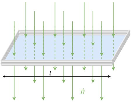
The square coil of Abbildung 5 has sides $l=0.25m$ long and is tightly wound with $N=200$ turns of wire. The resistance of the coil is $R=5.0\Omega$. The coil is placed in a spatially uniform magnetic field. The field is directed perpendicular to the face of the coil and whose magnitude is decreasing at a rate $dB/dt=−0.040T/s$.
- What is the magnitude of the potential difference induced in the coil?
- What is the magnitude of the current circulating through the coil?
Abb. 5: A square coil with N turns of wire with uniform magnetic field B directed in the downward direction, perpendicular to the coil
Strategy
The surface $\vec{A}$ is perpendicular to area covering the loop. We will choose this to be pointing downward so that $\vec{B⃗}$ is parallel to $\vec{A}$ and that the flux turns into multiplication of magnetic field times area. The area of the loop is not changing in time, so it can be factored out of the time derivative, leaving the magnetic field as the only quantity varying in time. Lastly, we can apply Ohm’s law once we know the induced potential difference to find the current in the loop.
Solution
The flux through one turn is
\begin{align*} \Phi_m = B \cdot A \end{align*}
We can calculate the magnitude of the potential difference $|U_{ind}|$ from Faraday’s law:
\begin{align*} |U_{ind}| &= |-{{d}\over{dt}}(N \cdot \Phi_m)| \\ &= -N \cdot {{d}\over{dt}} (B \cdot A) \\ &= -N \cdot l^2 \cdot {{dB}\over{dt}} \\ &= (200)(0.25m)^2(0.040 T/s) \\ &= 0.50 V \end{align*}
The magnitude of the current induced in the coil is
\begin{align*} |I| &= {{ |u_{ind}|}\over{R}} \\ &= {{0.50V}\over{5.0\Omega}} = 0.10A \\ \end{align*}
Task 4.1.2 Magnetic Field Strength around a horizontal straight Conductor
A closely wound coil has a radius of $4.0 cm$, $50$ turns, and a total resistance of $40\Omega$.
At what rate must a magnetic field perpendicular to the face of the coil change in order to produce Joule heating in the coil at a rate of $2.0 mW$?
Solution
$1.1 T/s$
4.2 Lenz Law
The direction in which the induced potential difference drives current around a wire loop can be found through the negative sign. However, it is usually easier to determine this direction with Lenz’s law, named in honor of its discoverer, Heinrich Lenz (1804–1865). (Faraday also discovered this law, independently of Lenz.) We state Lenz’s law as follows:
<callout icon=„fa fa-exclamation“ color=„red“ title=„Notice:“> Lenz's Law
The direction of the induced potential difference drives current around a wire loop to always oppose the change in magnetic flux that causes the potential difference.
Lenz’s law can also be considered in terms of conservation of energy. If pushing a magnet into a coil causes current, the energy in that current must have come from somewhere. If the induced current causes a magnetic field opposing the increase in field of the magnet we pushed in, then the situation is clear. We pushed a magnet against a field and did work on the system, and that showed up as current. If it were not the case that the induced field opposes the change in the flux, the magnet would be pulled in produce a current without anything having done work. Electric potential energy would have been created, violating the conservation of energy.
To determine an induced potential difference $u_{ind}$, you first calculate the magnetic flux $\Phi_m$ and then obtain $d\Phi_m / dt$. The magnitude of $u_{ind}$ is given by
\begin{align*} |u_{ind}| &= |-{{d}\over{dt}}(\Phi_m)| \end{align*}
Finally, you can apply Lenz’s law to determine the sense of $u_{ind}$. This will be developed through examples that illustrate the following problem-solving strategy.
Notice:
Problem-Solving Strategy: Lenz’s LawTo use Lenz’s law to determine the directions of induced potential difference, currents and magnetic fields:
- Make a sketch of the situation for use in visualizing and recording directions.
- Determine the direction of the applied magnetic field $\vec{B}$.
- Determine whether its magnetic flux is increasing or decreasing.
- Now determine the direction of the induced magnetic field $\vec{B_{ind}}$. The induced magnetic field tries to reinforce a magnetic flux that is decreasing or opposes a magnetic flux that is increasing. Therefore, the induced magnetic field adds or subtracts to the applied magnetic field, depending on the change in magnetic flux.
- Use right-hand rule to determine the direction of the induced current $i_{ind}$ that is responsible for the induced magnetic field $\vec{B_{ind}}$.
- The direction (or polarity) of the induced potential difference can now drive a conventional current in this direction.
Let’s apply Lenz’s law to the system of Abbildung ##. We designate the “front” of the closed conducting loop as the region containing the approaching bar magnet, and the “back” of the loop as the other region. The north pole of the magnet moves toward the loop. Therefore, the flux through the loop due to the field of the magnet increases because the strength of field lines directed from the front to the back of the loop is increasing. A current is consequently induced in the loop. By Lenz’s law, the direction of the induced current must be such that its own magnetic field is directed in a way to oppose the changing flux caused by the field of the approaching magnet. Hence, the induced current circulates so that its magnetic field lines through the loop are directed from the back to the front of the loop. By the rigth hand rule, place your thumb pointing against the magnetic field lines, which is toward the bar magnet. Your fingers wrap in a counterclockwise direction as viewed from the bar magnet. Alternatively, we can determine the direction of the induced current by treating the current loop as an electromagnet that opposes the approach of the north pole of the bar magnet. This occurs when the induced current flows as shown, for then the face of the loop nearer the approaching magnet is also a north pole.
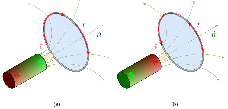
Part (b) of the figure shows the south pole of a magnet moving toward a conducting loop. In this case, the flux through the loop due to the field of the magnet increases because the number of field lines directed from the back to the front of the loop is increasing. To oppose this change, a current is induced in the loop whose field lines through the loop are directed from the front to the back. Equivalently, we can say that the current flows in a direction so that the face of the loop nearer the approaching magnet is a south pole, which then repels the approaching south pole of the magnet. By the rigth hand rule, your thumb points away from the bar magnet. Your fingers wrap in a clockwise fashion, which is the direction of the induced current.
4.3 Motional Induction
Magnetic flux depends on three factors:
- the strength of the magnetic field,
- the area through which the field lines pass, and
- the orientation of the field with the surface area.
If any of these quantities varies, a corresponding variation in magnetic flux occurs.
So far, we’ve only considered flux changes due to a changing field. Only the causing magnet was moving. This type of induction is called static induction (or stationary induction, in German: Ruheinduktion).
Now we look at another possibility: a changing area through which the field lines pass including a change in the orientation of the area. This leads us to motional induction
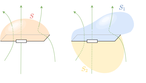
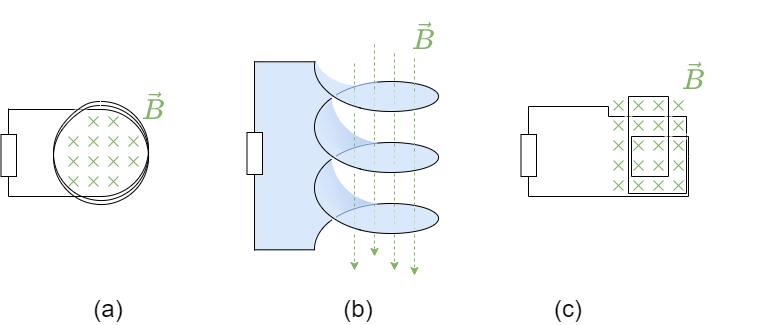
Two examples of this type of flux change are represented in Abbildung 7.
- In part (a), the magnetic flux changes as a loop moves into a magnetic field. The flux through the rectangular loop increases as it moves into the magnetic field,
- In part (b), magnetic flux changes as a loop rotates in a magnetic field. The flux through the rotating coil varies with the angle $\varphi$.
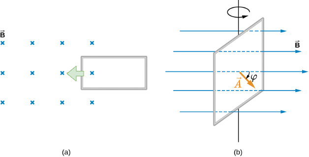
It’s interesting to note that what we perceive as the cause of a particular flux change actually depends on the frame of reference we choose. For example, if you are at rest relative to the moving coils of Abbildung 7 (b), you would see the flux vary because of a changing magnetic field. In part (a), the field moves from left to right in your reference frame, and in part (b), the field is rotating. It is often possible to describe a flux change through a coil that is moving in one particular reference frame in terms of a changing magnetic field in a second frame, where the coil is stationary. However, reference-frame questions related to magnetic flux are beyond this introduction. We’ll avoid such complexities by always working in a frame at rest relative to the laboratory and explain flux variations as due to either a changing field or a changing area.
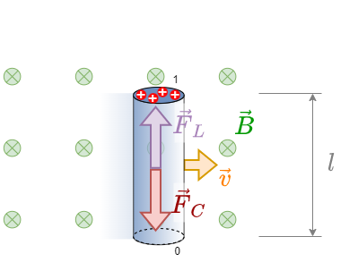
Single Rod
The first step to investigate the motional induction is shown in Abbildung 8: a single conducting rod with the length $\vec{l}$ which is moving with a constant velocity $\vec{v}$ through a homogenous magnetic field $\vec{B} \perp \vec{v} \perp \vec{l}$.
- The charges in the rod experience the Lorentz force $\vec{F}_L$.
- By this force, the positive charges move to one end of the rod and the negative to the other one.
- The separted charges create a patential difference and by this a Coulomb force $\vec{F}_C$ onto the charges within the rod.
- For a constant speed, the Lorentz force onto charges in the rod must have the same magnitude as the Coulomb force.
This leads to:
\begin{align*} \vec{F}_C &= - \vec{F}_L \\ q \cdot \vec{E}_{ind} &= - q \cdot \vec{v} \times \vec{B} \\ \vec{E}_{ind} &= - \vec{v} \times \vec{B} \\ \end{align*}
The induced potential difference in the rod will be:
\begin{align*} U_{ind} &= \int_l \vec{E}_{ind} \cdot d \vec{s} \\ &= - \int^0_1 \vec{v} \times \vec{B} \cdot d \vec{s} \\ \end{align*}
For constant $|\vec{v}|$ and $|\vec{B}|$ this leads to: \begin{align*} U_{ind} &= - v \cdot B \cdot l \\ \end{align*}
Rod in Circuit
Now let’s look at the conducting rod pulled in a circuit, changing magnetic flux. The area enclosed by the circuit '0123' of Abbildung 9 is $l\cdot x$ and is perpendicular to the magnetic field.
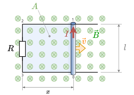
The velocity of the rod is $v=dx/dt$. So the induced potential difference will get \begin{align*} U_{ind} &= - v \cdot B \cdot l \\ &= - {{dx}\over{dt}} \cdot B \cdot l \\ &= - {{d}\over{dt}} \cdot B \cdot l \cdot x \\ &= - {{d}\over{dt}} \cdot B \cdot A \\ &= - {{d}\over{dt}} \cdot \Phi_m \\ \end{align*}
This is an alternative way to deduce Faraday's Law.
The current $I_{ind}$ induced in the given circuit is $U_{ind}$ divided by the resistance $R$
\begin{align*} I_{ind} = {{v \cdot B \cdot l }\over{R}} \end{align*}
Furthermore, the direction of the induced potential difference satisfies Lenz’s law, as you can verify by inspection of the figure.
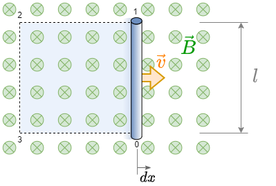
The situation of the single rod can be interpreted in the following way: We can calculate a motionally induced potential difference with Faraday’s law even when an actual closed circuit is not present. We simply imagine an enclosed area whose boundary includes the moving conductor, calculate $\Phi_m$ , and then find the potential difference from Faraday’s law. For example, we can let the moving rod of Abbildung 10 be one side of the imaginary rectangular area represented by the dashed lines. The area of the rectangle is $A=lx$, so the magnetic flux through it is $\Phi= B\cdot lx$. Differentiating this equation, we obtain
\begin{align*} U_{ind} &= - {{d}\over{dt}} \cdot \Phi_m \\ &= - B \cdot l \cdot {{dx}\over{dt}} \\ &= - B \cdot l \cdot v \\ \end{align*}
which is identical to the potential difference between the ends of the rod that we determined earlier.
Task 4.3.1 Calculating the Large Motional Potential difference of an Object in Orbit
Calculate the potential difference motional induced along a $20.0 km$ conductor moving at an orbital speed of $7.80 km/s$ perpendicular to Earth’s $5.00 \cdot 10^{-5}T$ magnetic field.
Strategy
This is a great example of using the equation motional $U_{ind} = - B \cdot l \cdot v$
Solution
Entering the given values into $U_{ind} = - B \cdot l \cdot v$ gives
\begin{align*} U_{ind} &= - {{d}\over{dt}} \cdot \Phi_m \\ &= - (5.00 \cdot 10^{-5}T)(20.0 \cdot 10^{3}m)(7.80\cdot 10^{3}m/s) \\ &= - 7.80 \cdot 10^3 V \\ \end{align*}
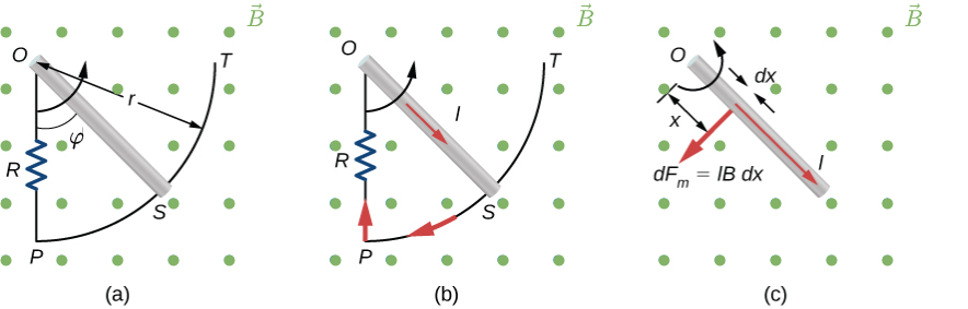
Task 4.3.2 A Metal Rod Rotating in a Magnetic Field
Part (a) of Abbildung 11 shows a metal rod OS that is rotating in a horizontal plane around point O. The rod slides along a wire that forms a circular arc PST of radius $r$. The system is in a constant magnetic field $\vec{B}$ that is directed out of the page.
If you rotate the rod at a constant angular velocity $\omega$, what is the current $I_{ind}$ in the closed loop OPSO? Assume that the resistor $R$ furnishes all of the resistance in the closed loop.
Strategy
The magnetic flux is the magnetic field times the area of the quarter circle or $A = r^2 \varphi /2$. When finding the potential difference through Faraday’s law, all variables are constant in time but $\varphi$, with $\omega = d\varphi/dt$. To calculate the work per unit time, we know this is related to the torque times the angular velocity. The torque is calculated by knowing the force on a rod and integrating it over the length of the rod.
Solution
From geometry, the area of the loop OPSO is $A=r^2\varphi /2$ . Hence, the magnetic flux through the loop is
\begin{align*} \Phi_m &= B\cdot A \\ &= B\cdot {{r^2\varphi}\over{2}} \\ \end{align*}
Differentiating with respect to time and using $\omega = d\varphi/dt$ , we have
\begin{align*} U_{ind} &= |{{d}\over{dt}} \cdot \Phi_m | \\ &= B\cdot {{r^2\omega}\over{2}} \end{align*}
When divided by the resistance $R$ of the loop, this yields for the magnitude of the induced current
\begin{align*} I_{ind} &= {{|U_{ind}|}\over{R}} \\ &= B\cdot {{r^2\omega}\over{2R}} \end{align*}
As $\varphi$ increases, so does the flux through the loop due to $\vec{B}$. To counteract this increase, the magnetic field due to the induced current must be directed into the page in the region enclosed by the loop. Therefore, as part (b) of Abbildung 11 illustrates, the current circulates clockwise.
Task 4.3.3 A Rectangular Coil Rotating in a Magnetic Field
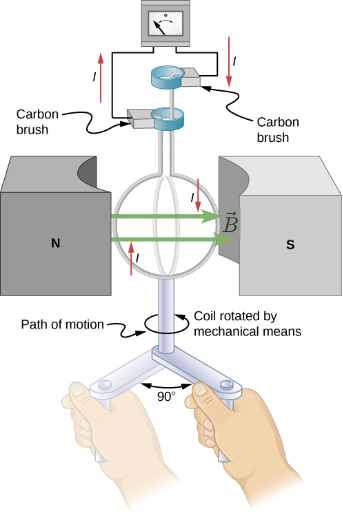
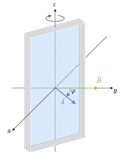
The following example is the basis for an electric generator: A rectangular coil of area $A$ and $N$ turns is placed in a uniform magnetic field $\vec{B}$, as shown in Abbildung 12. The coil is rotated about the $z$-axis through its center at a constant angular velocity $\omega$.
Obtain an expression for the induced potential difference $U_{ind}$ in the coil.
Strategy
According to the diagram, the angle between the surface vector $\vec{A}$ and the magnetic field $\vec{B}$ is $\varphi$. The dot product of $\vec{A} \cdot \vec{B}$ simplifies to only the $cos \varphi$ component of the magnetic field times the area, namely where the magnetic field projects onto the unit surface vector $\vec{A}$. The magnitude of the magnetic field and the area of the loop are fixed over time, which makes the integration simplify quickly. The induced potential difference is written out using Faraday’s law.
Solution
When the coil is in a position such that its surface vector $\vec{A}$ makes an angle $\varphi$ with the magnetic field $\vec{B}$ the magnetic flux through a single turn of the coil is
\begin{align*} \Phi_m &= \iint \vec{B} d\vec{A} \\ &= BA\cdot cos \varphi \\ \end{align*}
From Faraday’s law, the induced potential difference in the coil is
\begin{align*} u_{ind} &= - N |{{d}\over{dt}} \Phi_m \\ &= NBA \cdot sin \varphi \cdot {{d\varphi}\over{dt}} \end{align*}
The constant angular velocity is $\omega = d\varphi/dt$. The angle $\varphi$ represents the time evolution of the angular velocity or $\omega t$. This is changes the function to time space rather than $\varphi$. The induced potential difference therefore varies sinusoidally with time according to
\begin{align*} u_{ind} &= U_{ind,0} \cdot sin \omega t \end{align*}
where $U_{ind,0} = NBA\omega$.
Task 4.3.4 Calculating the Potential Difference Induced in a Generator Coil
The generator coil shown in Abbildung 13 is rotated through one-fourth of a revolution (from θ=0o to θ=90o ) in 15.0 ms. The 200-turn circular coil has a 5.00-cm radius and is in a uniform 0.80-T magnetic field.
What is the value of the induced potential difference?
Abb. 13: When this generator coil is rotated through one-fourth of a revolution, the magnetic flux changes from its maximum to zero, inducing an potential difference.
Strategy
Faraday’s law of induction is used to find the potential difference induced:
\begin{align*} u_{ind} &= - N {{d \Phi_m}\over{dt}} \end{align*}
We recognize this situation as the same one in the task before. According to the diagram, the projection of the surface vector $\vec{A}$ to the magnetic field is initially ${A}\cdot cos \varphi$ and this is inserted by the definition of the dot product. The magnitude of the magnetic field and area of the loop are fixed over time, which makes the integration simplify quickly. The induced potential difference is written out using Faraday’s law:
\begin{align*} u_{ind} &= N B \cdot sin \varphi \cdot {{d \varphi}\over{dt}} \end{align*}
Solution
We are given that $N=200$, $B=0.80T$ , $\varphi = 90°$ , $d\varphi=90°=\pi/2$ , and $dt=15.0ms$ .
The area of the loop is
\begin{align*} a = \pi r^2 = 3.14 \cdot (0.0500m)^2 = 7.85 \cdot 10^{-3} m^2 \end{align*}
Entering this value gives
\begin{align*} U_{ind} &= 200 \cdot (7.85 \cdot 10^{-3} m^2) \cdot sin 90° \cdot {{\pi /2}\over{15.0 \cdot 10^{-3} s}} = 131 V \end{align*}
4.4 Self-Induction
linked Flux
When looking onto the magnetic field in a coil multiple windings capture the passing flux, see Abbildung 14. Each winding will create a potential difference.
The resulting voltage is then given by the sum of the induced potential differences in each winding.
\begin{align*} u_{ind} &= - {{d \Phi_{sum}}\over{dt}} \\ &= - \sum_{i=1}^n {{d \Phi_{i}}\over{dt}} \\ \end{align*}
The linked flux $\Psi$ is defined as the resulting flux given by the sum of the partial fluxes of the closed ciruit.
\begin{align*} \Psi &= \sum_{i=1}^n \Phi_{i}} \\ \end{align*}
The linked flux simplifies the induced voltage of a coil to:
\begin{align*} u_{ind} &= - N \cdot {{d \Phi}\over{dt}} \\ &= - {{d \Psi}\over{dt}} \\ \end{align*}
Self-Induction
Up to now, we investigated the induction of voltages and currents based on the change of an external flux $d\Psi / dt$. For the induced current $i_{ind}$, we found that it counter acts the change of the external flux (Lenz law).
But what happens, when there is no external field - only a coil which creates the flux change itself?
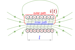
The created field density of the coil can be derived from Ampere's Circuital Law
\begin{align*} \theta(t) &= \int \vec{H}(t) \cdot d\vec{s} \\ &= \int \vec{H}_{inner}(t) \cdot d\vec{s} &+ \int \vec{H}_{ounter}(t) \cdot d\vec{s} \\ &= \int \vec{H}(t) \cdot d\vec{s} &+ 0 \\ &= {H}_{l}(t) \cdot l \\ \end{align*}
With magnetic voltage $\theta(t) = N \cdot i$ this lead to the magnetic flux density $B(t)$
\begin{align*} N \cdot i &= {H}_{l}(t) \cdot l \\ {H}(t) &= {{N \cdot i }\over {l}} \\ {B}(t) &= \mu \cdot {{N \cdot i }\over {l}} \\ \end{align*}
Based on the magnetic flux density $B(t)$ it is possible to calculate the flux $\Phi$:
\begin{align*} \Phi(t) &= \iint_A \vec{B}(t) \cdot d\vec{A} \\ &= \iint_A \mu \cdot {{N \cdot i }\over {l}} \cdot dA \\ &= \mu \cdot {{N \cdot i }\over {l}} \cdot A \\ &= \mu \cdot {{N \cdot i }\over {l}} \cdot {{\pi D^2}\over{4}} \\ \end{align*}
Mutual Induction
4.5 Inductivity
- Linked flux (see chapter 3.)
- self-induction
- formulas of different inductor types